Download
1 / 28
280 likes | 400 Views
Describing Bivariate Relationships. Chapter 3 Summary YMS AP Stats. 3.1 Response Vs. Explanatory Variables. Response variable measures an outcome of a study, explanatory variable helps explain or influences changes in a response variable (like independent vs. dependent).

E N D
Describing Bivariate Relationships • Chapter 3 Summary • YMS • AP Stats
3.1 Response Vs. Explanatory Variables • Response variable measures an outcome of a study, explanatory variable helps explain or influences changes in a response variable (like independent vs. dependent). • Calling one variable explanatory and the other response doesn’t necessarily mean that changes in one CAUSE changes in the other. • Ex: Alcohol and Body temp: One effect of Alcohol is a drop in body temp. To test this, researches give several amounts of alcohol to mice and measure each mouse’s body temp change. What are the explanatory and response variables?
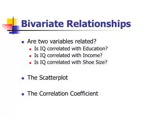
Scatterplots • Scatterplot shows the relationship between two quantitative variables measured on the same individuals. • Explanatory variables along X axis, Response variables along Y. • Each individual in data appears as the point in the plot fixed by the values of both variables for that individual. • Example:
Examining Scatterplots Overall pattern • Direction • Form • Strength • Outliers or deviations
Interpreting Scatterplots • Direction: in previous example, the overall pattern moves from upper left to lower right. We call this a negative association. • Form: The form is slightly curved and there are two distinct clusters. What explains the clusters? (ACT States) • Strength: The strength is determined by how closely the points follow a clear form. The example is only moderately strong. • Outliers: Do we see any deviations from the pattern? (Yes, West Virginia, where 20% of HS seniors take the SAT but the mean math score is only 511).
Calculator Scatterplot • Enter the Degree-Days in L1 and Gas in L2 • Next specify scatterplot in Statplot menu (first graph). X list L1 Y List L2 (explanatory and response) • Use ZoomStat. • Notice that their are no scales on the axes and they aren’t labeled. If you are copying your graph to your paper, make sure you scale and label the Axis (use Trace)
Correlation r • The Correlation measures the direction and strength of the linear relationship between 2 variables. • Formula- (don’t need to memorize or use): r = • In Calc: Go to Catalog (2nd, zero button), go to DiagnosticOn, enter, enter. You only have to do this ONCE! Once this is done: • Enter data in L1 and L2 (you can do calc-2 var stats if you want the mean and sd of each) • Calc, LinReg (A + Bx) enter
Interpreting Correlation • Caution- our eyes can be fooled! Our eyes are not good judges of how strong a linear relationship is. The 2 scatterplots depict the same data but drawn with a different scale. Because of this we need a numerical measure to supplement the graph.
Interpreting r • The absolute value of r tells you the strength of the association (0 means no association, 1 is a strong association) • The sign tells you whether it’s a positive or a negative association. So r ranges from -1 to +1 • Note- it makes no difference which variable you call x and which you call y when calculating correlation, but stay consistent! • Because r uses standardized values of the observations, r does not change when we change the units of measurement of x, y, or both. (Ex: Measuring height in inches vs. ft. won’t change correlation with weight) • values of -1 and +1 occur ONLY in the case of a perfect linear relationship , when the variables lie exactly along a straight line.
Examples 1. Correlation requires that both variables be quantitative 2. Correlation measures the strength of only LINEAR relationships, not curved...no matter how strong they are! 3. Like the mean and standard deviation, the correlation is not resistant: r is strongly affected by a few outlying observations. Use r with caution when outliers appear in the scatterplot 4. Correlation is not a complete summary of two-variable data, even when the relationship is linear- always give the means and standard deviations of both x and y along with the correlation.
3.3- least squares regression Text The slope here B = .00344 tells us that fat gained goes down by .00344 kg for each added calorie of NEA according to this linear model. Our regression equation is the predicted RATE OF CHANGE in the response y as the explanatory variable x changes. The Y intercept a = 3.505kg is the fat gain estimated by this model if NEA does not change when a person overeats.
Prediction • We can use a regression line to predict the response y for a specific value of the explanatory variable x.
LSRL • In most cases, no line will pass exactly through all the points in a scatter plot and different people will draw different regression lines by eye. • Because we use the line to predict y from x, the prediction errors we make are errors in y, the vertical direction in the scatter plot • A good regression line makes the vertical distances of the points from the line as small as possible • Error: Observed response - predicted response
Equation of LSRL • Example: The Sanchez household is about to install solar panels to reduce the cost of heating their house. In order to know how much the panels help, they record their consumption of natural gas before the panels are installed. Gas consumption is higher in cold weather, so the relationship between outside temp and gas consumption is important.
Facts about Least-Squares regression • The distinction between explanatory and response variables is essential in regression. If we reverse the roles, we get a different least-squares regression line. • There is a close connection between corelation and the slope of the LSRL. Slope is r times Sy/Sx. This says that a change of one standard deviation in x corresponds to a change of 4 standard deviations in y. When the variables are perfectly correlated (4 = +/- 1), the change in the predicted response y hat is the same (in standard deviation units) as the change in x. • The LSRL will always pass through the point (X bar, Y Bar) • r squared is the fraction of variation in values of y explained by the x variable
Describe the direction, form, and strength of the relationship • Positive, linear, and very strong • About how much gas does the regression line predict that the family will use in a month that averages 20 degree-days per day? • 500 cubic feet per day • How well does the least-squares line fit the data?
R squared- Coefficient of determination If all the points fall directly on the least-squares line, r squared = 1. Then all the variation in y is explained by the linear relationship with x. So, if r squared = .606, that means that 61% of the variation in y among individual subjects is due to the influence of the other variable. The other 39% is “not explained”. r squared is a measure of how successful the regression was in explaining the response
3.3 Influences • Correlation r is not resistant. Extrapolation is not very reliable. One unusual point in the scatterplot greatly affects the value of r. LSRL also not resistant. • A point extreme in the x direction with no other points near it pulls the line toward itself. This point is influential.
Lurking Variables- Beware! • Example: A college board study of HS grads found a strong correlation between math minority students took in high school and their later success in college. News articles quoted the College Board saying that “math is the gatekeeper for success in college”. • But, Minority students from middle-class homes with educated parents no doubt take more high school math courses. They are also more likely to have a stable family, parents who emphasize education, and can pay for college etc. These students would likely succeed in college even if they took fewer math courses. The family background of students is a lurking variable that probably explains much of the relationship between math courses and college success.
Residuals • The error of our predictions, or vertical distance from predicted Y to observed Y, are called residuals because they are “left-over” variation in the response. One subject’s NEA rose by 135 calories. That subject gained 2.7 KG of fat. The predicted gain for 135 calories is Y hat = 3.505- .00344(135) = 3.04 kg The residual for this subject is y - yhat = 2.7 - 3.04 = -.34 kg
Residual Plot • The sum of the least-squares residuals is always zero. • The mean of the residuals is always zero, the horizontal line at zero in the figure helps orient us. This “residual = 0” line corresponds to the regression line
Examining Residual Plot • Residual plot should show no obvious pattern. A curved pattern shows that the relationship is not linear and a straight line may not be the best model. • Residuals should be relatively small in size. A regression line in a model that fits the data well should come close” to most of the points. • A commonly used measure of this is the standard deviation of the residuals, given by: For the NEA and fat gain data, S =
Residuals List on Calc • If you want to get all your residuals listed in L3 highlight L3 (the name of the list, on the top) and go to 2nd- stat- RESID then hit enter and enter and the list that pops out is your resid for each individual in the corresponding L1 and L2. (if you were to create a normal scatter plot using this list as your y list, so x list: L1 and Y list L3 you would get the exact same thing as if you did a residual plot defining x list as L1 and Y list as RESID as we had been doing). This is a helpful list to have to check your work when asked to calculate an individuals residual.
Residual Plot on Calc • Produce Scatterplot and Regression line from data (lets use BAC if still in there) • Turn all plots off • Create new scatterplot with X list as your explanatory variable and Y list as residuals (2nd stat, resid) • Zoom Stat
Bivariate Relationships • What is Bivariate data? • When exploring/describing a bivariate (x,y) relationship: • Determine the Explanatory and Response variables • Plot the data in a scatterplot • Note the Strength, Direction, and Form • Note the mean and standard deviation of x and the mean and standard deviation of y • Calculate and Interpret the Correlation, r • Calculate and Interpret the Least Squares Regression Line in context. • Assess the appropriateness of the LSRL by constructing a Residual Plot.