Download
1 / 37
410 likes | 905 Views
Syntactic Analysis and Parsing . (Based on: Compilers, Principles, Techniques and Tools , by Aho, Sethi and Ullman, 1986). Compilers. A Compiler is a program that reads a program written in one language (the source language ) and translates it into another (the target language )

E N D
Syntactic Analysis and Parsing (Based on: Compilers, Principles, Techniques and Tools, by Aho, Sethi and Ullman, 1986)
Compilers • A Compiler is a program that reads a program written in one language (the source language) and translates it into another (the target language) • A compiler operates in phases, each of which transforms the source program from one representation to the other Source program Lexical Analyzer Syntax Analyzer Semantic Analyzer Intermediate Code Generator Code Optimizer Code Generator Target Program • The part of the compiler we will focus on in this part of the course is the Syntax Analyzer or Parser.
Parsing • Parsing is the process of determining whether a string of tokens can be generated by a grammar. • Most parsing methods fall into one of two classes, called the top-downand bottom-up methods. • In top-down parsing, construction starts at the root and proceeds to the leaves. In bottom-up parsing, construction starts at the leaves and proceeds towards the root. • Efficient top-down parsers are easy to build by hand. • Bottom-up parsing, however, can handle a larger class of grammars. They are not as easy to build, but tools for generating them directly from a grammar are available.
Part ITop Down Parsing • Basic Ideas behind Top-Down Parsing • Predictive Parsers • Left Recursive Grammars • Left Factoring a grammar • Constructing a Predictive Parser • LL(1) Grammars
Basic Idea behind Top-Down Parsing • Top-Down Parsing is an attempt to find a left-most derivation for an input string • Example: S cAd Find a derivation for A ab | a for w cad S S Backtrack S / | \ / | \ / | \ c A d c A d c A d / \ | a b a
Predictive Parser: Generalities • In many cases, by carefully writing a grammar—eliminating left recursion from it and left factoring the resulting grammar—we can obtain a grammar that can be parsed by a recursive-descent parser that needs no backtracking. • Such parsers are called predictive parsers.
Left Recursive Grammars I • A grammar is left recursive if it has a nonterminal A such that there is a derivation A Aα, for some string α • Top-down parsers can loop forever when facing a left-recursive rules. Therefore, such rules need to be eliminated. • A left-recursive rule such as A A α | β can be eliminated by replacing it by: • A β R where R is a new non-terminal • R α R | є and є is the empty string • The new grammar is right-recursive
Left-Recursive Grammars II • The general procedure for removing direct left recursion—recursion that occurs in one rule—is the following: • Group the A-rules as A Aα1 |… | Aαm | β1 | β2 |…| βn where none of the β’s begins with A • Replace the original A-rules with • A β1A’ | β2 A’ | … | βn A’ • A’ α1 A’ | α2 A’ | … | αm A’ • This procedure will not eliminate indirect left recursion of the kind: • A BaA • B Ab [Another procedure exists that is not given here] • Direct or Indirect Left-Recursion is problematic for all top-down parsers. However, it is not a problem for bottom-up parsing algorithms.
Left-Recursive Grammars III • Here is an example of a (directly) left-recursive grammar: E E + T | T T T * F | F F ( E ) | id • This grammar can be re-written as the following non left-recursive grammar: E T E’ E’ + TE’ | є T F T’ T’ * F T’ | є F (E) | id
Left-Factoring a Grammar I • Left Recursion is not the only trait that disallows top-down parsing. • Another is whether the parser can always choose the correct Right Hand Side on the basis of the next token of input, using only the first token generated by the leftmost nonterminal in the current derivation. • To ensure that this is possible, we need to left-factor the non left-recursive grammar generated in the previous step.
Left-Factoring a Grammar II • Here is the procedure used to left-factor a grammar: • For each non-terminal A, find the longest prefix α common to two or more of its alternatives. • Replace all the A productions: A αβ1 | αβ2 … | αβn | γ (where γ represents all alternatives that do not begin with α) • By: A α A’ | γ A’ β1 | β2 | … | βn
Left-Factoring a Grammar III • Here is an example of a common grammar that needs left factoring: S iEtS | iEtSeS | a E b ( i stands for “if”; t stands for “then”; and e stands for “else”) • Left factored, this grammar becomes: S iEtSS’ | a S’ eS | є E b
Predictive Parser: Details • The key problem during predictive parsing is that of determining the production to be applied for a non-terminal. • This is done by using a parsing table. • A parsing table is a two-dimensional array M[A,a] where A is a non-terminal, and a is a terminal or the symbol $, menaing “end of input string”. • The other inputs of a predictive parser are: • The input buffer, which contains the string to be parsed followed by $. • The stack which contains a sequence of grammar symbols with, initially, $S (end of input string and start symbol) in it.
Predictive Parser: Informal Procedure • The predictive parser considers X, the symbol on top of the stack, and a, the current input symbol. It uses, M, the parsing table. • If X=a=$ halt and return success • If X=a≠$ pop X off the stack and advance input pointer to the next symbol • If X is a non-terminal Check M[X,a] • If the entry is a production rule, then replace X on the stack by the Right Hand Side of the production • If the entry is blank, then halt and return failure
Predictive Parser: An Example Parsing Table Algorithm Trace
Constructing the Parsing Table I: First and Follow • First(α) is the set of terminals that begin the strings derived from α. Follow(A) is the set of terminals a that can appear to the right of A. First and Follow are used in the construction of the parsing table. • Computing First: • If X is a terminal, then First(X) is {X} • If X є is a production, then add є to First(X) • If X is a non-terminal and X Y1 Y2 … Yk is a production, then place a in First(X) if for some i, a is in First(Yi) and є is in all of First(Y1)…First(Yi-1)
Constructing the Parsing Table II: First and Follow • Computing Follow: • Place $ in Follow(S), where S is the start symbol and $ is the input right endmarker. • If there is a production A αBβ, then everything in First(β) except for є is placed in Follow(B). • If there is a production A αB, or a production A αBβ where First(β) contains є, then everything in Follow(A) is in Follow(B) Example: E TE’ E’ +TE’ | є T FT’ T’ *FT’ | є F (E) | id First(E) = First(T) = First(F) = {(, id} First(E’) = {+, є} First(T’) = {*, є} Follow(E) = Follow(E’) = {),$} Follow(F)={+,*,),$} Follow(T) = Follow(T’) = {+,),$}
Constructing the Parsing Table III • Algorithm for constructing a predictive parsing table: • For each production A α of the grammar, do steps 2 and 3 • For each terminal a in First(α), add A α to M[A, a] • If є is in First(α), add A α to M[A, b] for each terminal b in Follow(A). If є is in First(α), add A α to M[A,b] for each terminal b in Follow(A). If є is in First(α) and $ is in Follow(A), add A α to M[A, $]. • Make each undefined entry of M be an error.
LL(1) Grammars • A grammar whose parsing table has no multiply-defined entries is said to be LL(1) • No ambiguous or left-recursive grammar can be LL(1). • A grammar G is LL(1) iff whenever A α | β are two distinct productions of G, then the following conditions hold: • For no terminal a do both α and β derive strings beginning with a • At most one of α and β can derive the empty string • If β can (directly or indirectly) derive є, then α does not derive any string beginning with a terminal in Follow(A).
Part IIBottom-Up Parsing • There are different approaches to bottom-up parsing. One of them is called Shift-Reduce parsing, which in turns has a number of different instantiations. • Operator-precedence parsing is one such method as is LR parsing which is much more general. • In this course, we will be focusing on LR parsing. LR Parsing itself takes three forms: Simple LR-Parsing (SLR) a simple but limited version of LR-Parsing; Canonical LR parsing, the most powerful, but most expensive version; and LALR which is intermediate in cost and power. Our focus will be on SLR-Parsing.
LR Parsing: Advantages • LR Parsers can recognize any language for which a context free grammar can be written. • LR Parsing is the most general non-backtracking shift-reduce method known, yet it is as efficient as ither shift-reduce approaches • The class of grammars that can be parsed by an LR parser is a proper superset of that that can be parsed by a predictive parser. • An LR-parser can detect a syntactic error as soon as it is possible to do so on a left-to-right scan of the input.
LR-Parsing: Drawback/Solution • The main drawback of LR parsing is that it is too much work to construct an LR parser by hand for a typical programming language grammar. • Fortunately, specialized tools to construct LR parsers automatically have been designed. • With such tools, a user can write a context-free grammar and have a parser generator automatically produce a parser for that grammar. • An example of such a tool is Yacc “Yet Another Compiler-Compiler”
LR Parsing Algorithms: Details I • An LR parser consists of an input, output, a stack, a driver program and a parsing table that has two parts: action and goto. • The driver program is the same for all LR Parsers. Only the parsing table changes from one parser to the other. • The program uses the stack to store a string of the form s0X1s1X2…Xmsm, where sm is the top of the stack. The Sk‘s are state symbols while the Xi‘s are grammar symbols. Together state and grammar symbols determine a shift-reduce parsing decision.
LR Parsing Algorithms: Details II • The parsing table consists of two parts: a parsing action function and a goto function. • The LR parsing program determines sm, the state on top of the stack and ai, the current input. It then consults action[sm, ai] which can take one of four values: • Shift • Reduce • Accept • Error
LR Parsing Algorithms: Details III • If action[sm, ai] = Shift s, where s is a state, then the parser pushes ai and s on the stack. • If action[sm, ai] = Reduce A β, then ai and sm are replaced by A, and, if s was the state appearing below ai in the stack, then goto[s, A] is consulted and the state it stores is pushed onto the stack. • If action[sm, ai] = Accept, parsing is completed • If action[sm, ai] = Error, then the parser discovered an error.
LR Parsing Example: The Grammar • E E + T • E T • T T * F • T F • F (E) • F id
SLR Parsing • Definition: An LR(0) item of a grammar G is a production of G with a dot at some position of the right side. • Example: A XYZ yields the four following items: • A .XYZ • A X.YZ • A XY.Z • A XYZ. • The production A є generates only one item, A . • Intuitively, an item indicates how much of a production we have seen at a given point in the parsing process.
SLR Parsing • To create an SLR Parsing table, we define three new elements: • An augmented grammar for G, the initial grammar. If S is the start symbol of G, we add the production S’ .S . The purpose of this new starting production is to indicate to the parser when it should stop parsing and accept the input. • The closure operation • The goto function
SLR Parsing:The Closure Operation • If I is a set of items for a grammar G, then closure(I) is the set of items constructed from I by the two rules: • Initially, every item in I is added to closure(I) • If A α . B β is in closure(I) and B γ is a production, then add the item B . γ to I, if it is not already there. We apply this rule until no more new items can be added to closure(I).
SLR Parsing:The Closure Operation – Example Original grammar Augmented grammar 0. E’ E • E E + T 1. E E + T • E T 2. E T • T T * F 3. E T * F • T F 4. T F • F (E) 5. F (E) • F id 6. F id Let I = {[E’ E]} then Closure(I)= { [E’ .E], [E .E + T], [E .T], [E .T*F], [T .F], [F .(E)] [F .id] }
SLR Parsing:The Goto Operation • Goto(I,X), where I is a set of items and X is a grammar symbol, is defined as the closure of the set of all items [A αX.β] such that [A α.Xβ] is in I. • Example: If I is the set of two items {E’ E.], [E E.+T]}, then goto(I, +) consists of E E + .T T .T * F T .F F .(E) F .id
SLR Parsing:Sets-of-Items Construction Procedure items(G’) C = {Closure({[S’ .S]})} Repeat For each set of items I in C and each grammar symbol X such that got(I,X) is not empty and not in C do add goto(I,X) to C Until no more sets of items can be added to C
Example: The Canonical LR(0) collection for grammar G I0: E’ .E I4: F (.E) I7: T T * .F E .E + T E .E + T F .(E) E .T E .T F .id T .T * F T .T * F I8: F (E.) T .F T .F E E.+T F .(E) F .(E) I9: E E + T. F .id F .id T T.* F I1: E’ E. I5: F id. I10: T T*F. E E.+T I6: E E+.T I11: F (E). I2: E T. T .T*F T T. * F T .F I3: T F. F .(E) F .id
Constructing an SLR Parsing Table • Construct C={I0, I1, … In} the collection of sets of LR(0) items for G’ • State i is constructed from Ii. The parsing actions for state i are determined as follows: • If [A α.aβ] is in Ii and goto(Ii,a) = Ij, then set action[i,a] to “shift j”. Here, a must be a terminal. • If [A α.] is in Ii, then set action[i, a] to “reduce A α” for all a in Follow(A); here A may not be S’. • If [S’ S.] is in Ii, then set action[i,$] to “accept” If any conflicting actions are generated by the above rules, we say that the grammar is not SLR(1). The algorithm then fails to produce a parser.
Constructing an SLR Parsing Table (cont’d) 3. The goto transitions for state i are constructed for all nonterminals A using the rule: If goto(Ii, A) = Ij, then goto[i, A] = j. 4. All entries not defined by rules (2) and (3) are made “error”. 5. The initial state of the parser is the one constructed from the set of items containing [S’ S]. See example in class