Download
1 / 38
380 likes | 484 Views
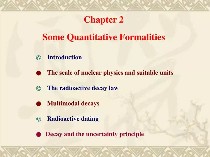
Chapter 2 Some Quantitative Formalities. ◎ Introduction ● The scale of nuclear physics and suitable units ◎ The radioactive decay law ● Multimodal decays ◎ Radioactive dating ● Decay and the uncertainty principle. § 2.1 The scale of nuclear physics and suitable units. Nuclear measurement

E N D
Chapter 2 Some Quantitative Formalities ◎Introduction ●The scale of nuclear physics and suitable units ◎The radioactive decay law ●Multimodal decays ◎Radioactive dating ●Decay and the uncertainty principle
§ 2.1 The scale of nuclear physics and suitable units • Nuclear measurement • cross-section --- collisions • spontaneous change --- decays •Geiger counter
Human’s Scale The scale of the known universe and the position of humans within it.
We need some convenient units to do nuclear calculations. The familiar SI units are not handy. Nuclear dimension ~ 10-15 m Nuclear masses ~ 10-27 kg
Convenient energy units Atomic Scale ~ eV Nuclear Scale ~ MeV (106 eV) Particle Scale ~ GeV (109 eV)
Useful units and their SI equivalence (1) E total energy plinear momentum Mrest mass c speed of light
§ 2.2 The radioactive decay law Suppose that at time t =0 we have an assembly of a number N(0) of X and at time t a number N(t) survive. Then (1) ω: the transition rate; The probability that a state of a system will make a transition to another state in a period of one second. It is sometimes referred as the decay constant.
(1) Hence (2) This is the radioactive decay law. It is a survival equation giving the number of the state X remaining unchanged until the time t. (3) τ is the mean life time of the state X.
(3) τ is the mean life time of the state X. Mean life time(or mean life) The average life time of an unstable state in a large sample of such states. It is also the time at which the number of states surviving is e-1 of the number present initially.
Decay Mean life Examples of decay processes and their mean lives.
The graphical form of the radioactive decay law showing the relation between mean life (τ) and the half-life (t1/2) (4)
The detection of radioactivity normally requires the detection of radiation emitted when a nucleus decay. Thus the total intensity detectable at time t is given by (5) (6) or The radioactivity detected by the intensity of particles emitted itself decays at the same rate as does the number of surviving nuclei.
These two equations are strictly probability relations and are subject to statistical fluctuations. Only in the limit of very large numbers do the statistical fluctuations become relatively small. (2) (6) σ: relative fluctuation
Units of radioactivity Curie (Ci) One curie is the amount of a radioactive material in which the number of disintegrations in one second is the same as that of one gram of pure radium(Ra). The number is 3.7 1010 s-1. Becquerel (Bq) One becquerel is the amount of a radioactive material in which the average number of disintegration in one second is one.
Examples of activities • The activity of one person weighing 70 kg is about • 10-7 Ci = 3.7 103 Bq mainly due to K-40and C-14. 2. The activity of one cubic meter of air in a dwelling house depends on the nature of the building material and of the ground below, and on the ventilation. It therefore varies, from below 100 Bq to 1000 Bq or higher, mainly due to a radon isotope (Rn-222) and its decay products. Another unit:sievert (Sv) The sievert is defined in a way which takes account of the susceptibility of human tissue to long term risk from radiation. One Sv is approximately 1 J of energy deposited per kilogram of absorbing material in the case of electrons and γ-rays.
The United States maximum permissible occupational whole body-dose is 50 millisieverts(mSv) per year.
The effect of certain radiation on a biological system depends on the absorbed doseDand on thequality factorQF of the radiation. The dose equivalentDEis obtained by multiplying these quantities together. SI unit
Radon Radiation risk: e.g. the Sievert unit of absorbed dose
§ 2.3 Multimodal decays Consider the case that two modes of decay are possible. f1: the branching fraction of α-decay f2: the branching fraction of β--decay There are two partial transition rates, ω1 and ω2, for the two decay modes separately. The total transition rate for decay of the parent nucleus is given by (7)
(7) and therefore (8) Its mean life time τ is therefore (9) and (10)
Fill in the last column of this table The decay of the K+ meson
§ 2.3 The radioactive dating Carbon dating Biological carbon comes from atmospheric CO2which contains the active 14C (decays to 14N) in the ratio of 1 atomic part in about 1012 of the stable isotope 12C. Once fixed biologically, the decay of the 14C causes a decline in this ratio with a half-life 0f 5730 years. The 14C is produced in the atmosphere by the action of cosmic rays and if we believe their intensity has not changed significantly (probably not true !)then the ratio 14C/ 12C at the time of biological fixing is the same as it was before 1945 (when atmospheric nuclear weapon testing injected unnatural 14Cinto the atmosphere) Thus an assumed ratio at biological fixing and a measured ratio at investigation will give the age of a biological specimen.
Rapa Nui Easter Island Carbon dating method has an evident uncertainness which has to do with the uncertainty of the assumed initial ratio. This uncertainty can be removed by calibrating against other methods of dating when applicable.
§ 2.4 Decay and the uncertainty principle Mass spectrum of μ+μ- pairs in the PHENIX detector showing clear evidence of the J/Ψ resonance. Image Courtesy PHENIX Collaboration.
Energy spectrum of 182Hf 182Hf with its half-life of about 9 million years is a long-lived radionuclide. It is very important for nuclear astrophysics research to detect minute amounts of 182Hf with AMS (erator mass spectrometry), a ultra-high sensitive nuclear analyzing technique. In present work, the procedures of sample preparation of HfF4 and decontamination of tungsten from the samples have been researched, and the detection efficiencies and energy spectrum of 182Hf have been measured at CIAE HI-13 tandem accelerator AMS facility. The main interference for the detection is the stable isobar 182W which can be significantly reduced by injecting negative ion of HfF5-. The ion source efficiency and accelerator transmission efficiency for 182Hf are 3×10⁻³ and 5×10⁻³, respectively, in CIAE AMS system. The energy spectrum of 182Hf standard sample, which has been measured with a semi-conductor detector, is showed in Fig.1. http://202.38.8.9/nianbao/english/english2004/5.htm
Γ A decaying state is a system with an uncertainty of lifetime equal to the mean life (ω-1) of that state. It follows that there is an uncertainty in the total energy given by (11) The uncertainty in energy of an excited state is reflected in the line shape of the radiation emitted in decay to the ground state.
Γ The shape is Lorentzian; it is given by (12) (13) E0 is the central energy and the expression gives the relative probability of finding an energy E. Γ is the full width at half height, so that Γ/2 is the energy uncertainty. The Lorentzian shape is the transform of the exponential time decay, yielding as expected from the uncertainty principle.
The discussion of “width” If a nucleus is in an excited state, it must discard excess energy it has by undergoing a decay. It is, however, impossible to predict when the decay will actually take place. As a result, there is an uncertainty in time Δt = τ associated with the existence of the excited state. Because of the limited lifetime, it is impossible for us to measure its energy to infinite precision. This phenomenon has an explanation in quantum mechanics!
Γ If we carry out the energy measurement for Nnuclei in the same excited state, there will be a distribution of the values obtained. If the value of the ith excited nucleus is Ei, the average <E>is given by (14) An idea of the spread in the measured values is provided by the square root of the variance, (15)
The Heisenberg uncertainty principle says that the product of Γ and τ is equal to Γ The quantity Γis known as the natural line width, or width for short, of a state. (13) It is also a way to indicate the transition probability of a state and is proportional to the inverse of the life time τ.
One can also relate Γ to the probability of finding the excited state at a specific energy. In terms of the wave functions, the decay constant ωmay be defined in the following way: (16) For a stationary state, the time-dependent wave function may be written as (17)
To carry such an expression over to a decaying (excited) state, the energy E must be changed into a complex quantity, (18) The time-dependent wave function now takes the form (19)
An excited state is the one without a definite energy its wave function should be a superposition of components having different energies, (20) where a(E) is the probability amplitude for finding the state at energy E. From equations (19) and (20)
so that (21) In the equation (21) we recognize that e-ωt/2 is the Fourier transform of a(E). Therefore (22)
Γ The probability for finding the excited state at energy E is given by the absolute square of the amplitude, (23) with (13) Lorentzian shape curve