Binomial Probability Distribution

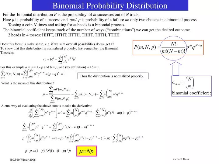
1. Binomial Probability Distribution For the binomial distribution P is the probability of m successes out of N trials. Here p is probability of a success and q=1-p is probability of a failure Þonly two choices in a binomial process. Tossing a coin N times and asking for m heads is a binomial process. The binomial coefficient keeps track of the number of ways (“combinations”) we can get the desired outcome. 2 heads in 4 tosses: HHTT, HTHT, HTTH, THHT, THTH, TTHH m=Np Richard Kass

2. What’s the variance of a binomial distribution? Using a trick similar to the one used for the average we find: Binomial Probability Distribution Detection efficiency and its “error”: Note: se, the “error in the efficiency” ®0 as e® 0 or e® 1. (This is NOT a gaussian s so don’t stick it into a Gaussian pdf to calculate probability) x x G G Richard Kass

3. Binomial Probability Distributions Richard Kass

4. Poisson Probability Distribution aradioactive decay anumber of Prussian soldiers kicked to death by horses per year per army corps! aquality control, failure rate predictions N>>m In a counting experiment if you observe m events: Richard Kass

5. Poisson Probability Distribution ln10!=15.10 10ln10-10=13.03 ®14% ln50!=148.48 50ln50-50=145.60®1.9% Not much difference between them here! Comparison of Binomial and Poisson distributions with mean m=1. Richard Kass

6. Counting the numbers of cosmic rays that pass through a detector in a 15 sec interval Poisson Probability Distribution Data is compared with a poisson using the measured average number of cosmic rays passing through the detector in eighty one 15 sec. intervals (m=5.4) Error bars are (usually) calculated using Öni (ni=number in a bin) Why? Assume we have N total counts and the probability to fall in bin i is pi. For a given bin we have a binomial distribution (you’re either in or out). The expected average number in a given bin is: Npi and the variance is Npi(1-pi)=ni(1-pi) If we have a lot of bins then the probability of a event falling into a bin is small so (1-pi) »1 In our example the largest pi =17/81=0.21 correction=(1-.21)1/2=0.88 poisson with m=5.4 number of occurrences number of cosmic rays in a 15 sec. interval Richard Kass

7. Gaussian Probability Distribution x It is very unlikely (<0.3%) that a measurement taken at random from a gaussian pdf will be more than ±3s from the true mean of the distribution. Richard Kass

8. Central Limit Theorem Why is the gaussian pdf so important ? Actually, the Y’s can be from different pdf’s! For CLT to be valid: m and s of pdf must be finite No one term in sum should dominate the sum Richard Kass

9. Best illustration of the CLT. a) Take 12 numbers (ri) from your computer’s random number generator b) add them together c) Subtract 6 d) get a number that is from a gaussian pdf ! Central Limit Theorem Computer’s random number generator gives numbers distributed uniformly in the interval [0,1] A uniform pdf in the interval [0,1] has m=1/2 and s2=1/12 A) 5000 random numbers B) 5000 pairs (r1+ r2) of random numbers Thus the sum of 12 uniform random numbers minus 6 is distributed as if it came from a gaussian pdf with m=0 and s=1. D) 5000 12-plets (r1+ ++r12) of random numbers. C) 5000 triplets (r1+ r2+ r3) of random numbers E) 5000 12-plets (r1+ ++r12-6)of random numbers. E Gaussian m=0 and s=1 In this case, 12 is close to ¥. -6 0 +6 Richard Kass

10. Central Limit Theorem • Example: An electromagnetic calorimeter is being made out of a sandwich of lead and plastic scintillator. There are 25 pieces of lead and 25 pieces of plastic, each piece is nominally 1 cm thick. The spec on the thickness is 0.5 mm and is uniform in [-0.5,0.5] mm. The calorimeter has to fit inside an opening of 51 cm. What is the probability that it won’t will fit? • Since the machining errors come from a uniform distribution with a well defined mean and variance the Central Limit Theorem is applicable: • The upper limit corresponds to many large machining errors, all +0.5 mm: • The lower limit corresponds to a sum of machining errors of 1 cm. • The probability for the stack to be greater than51 cm is: • There’s a 31% chance the calorimeter won’t fit inside the box! (and a 100% chance someone will get fired if it doesn’t fit inside the box…) Richard Kass

11. Case I) PDF does not have a well defined mean or variance. The Breit-Wigner distribution does not have a well defined variance! When Doesn’t the Central Limit Theorem Apply? Describes the shape of a resonance, e.g. K* Case II) Physical process where one term in the sum dominates the sum. i) Multiple scattering: as a charged particle moves through material it undergoes many elastic (“Rutherford”) scatterings. Most scattering produce small angular deflections (ds/dW~q-4) but every once in a while a scattering produces a very large deflection. If we neglect the large scatterings the angle qplane is gaussian distributed. The mean q depends on the material thickness & particle’s charge & momentum ii) The spread in range of a stopping particle (straggling). A small number of collisions where the particle loses a lot of its energy dominates the sum. iii) Energy loss of a charged particle going through a gas. Described by a “Landau” distribution (very long “tail”). Richard Kass