Download
1 / 41
420 likes | 608 Views
LEARNING ALGORITHMS for SERVO- MECHANISM TIME SUBOPTIMAL CONTROL. M. Alex í k , University of Žilina, Slovak Republic. 1 - Time Optimal Control - S witching F unction ( SwF ) 2 - Sliding Mode Control (SMC), Adaptive Sliding Mode Control

E N D
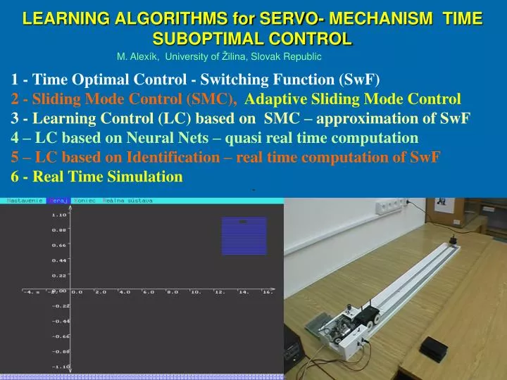
LEARNING ALGORITHMS for SERVO- MECHANISMTIMESUBOPTIMAL CONTROL M. Alexík, University of Žilina, Slovak Republic 1 - Time Optimal Control - Switching Function (SwF) 2 - Sliding Mode Control (SMC), Adaptive Sliding Mode Control 3 -Learning Control (LC) based on SMC – approximation of SwF 4 – LC based on Neural Nets – quasi real time computation 5 – LC based on Identification – real time computation of SwF 6 - Real Time Simulation
Laboratory Model of Servomechanism (6+1)x 0.6 kg Cart with variable load Spring Hand Control Time and position Display Load Load DC Drive with gear µP Atmel Communicationwith PC – RS 232 GOAL: Derivation of Time Optimal Control algorithm for Servomechanism with variable load. „Time Optimal (feedback) Control“ - „Sliding Mode Control“ – estimation of switching function (switchingcurved line, or approximation- only line, polynomial). For variable unknown load of servomechanism and time suboptimal control is necessary to apply learning algorithm for looking for switching function (curved line, line). Problem: Nonlinearities – variable fiction, two springs – non sensitivity in output variable M. Alexík, KEGA,06- 08, Žilina, Sept. 2008
Physical Model of Servomechanism real time simulation Km Tem[s] Colours Weights - cart Weights circular mecha- nism 0.085 1.0 Blue 1 0 Purple 0.058 1.5 1 2 0.046 1.75 Green 1 4 0.034 2.0 Brown 1 6 Km S(s) = Km = 1/b, Tem = m/b s(Tem s + 1) m = Weights(changeable), b = coef. of friction (changeable) then Km, Temarealso changeable = + x & ( t ) Ax ( t ) b u ( t ) - é é ù é ù ( ) e ( t ) w y ( t ) 1 = = = x (t) ê ê ú ê ú - x ( t ) e ( t ) y ( t ) & & ë û ë û ë 2 D/A converter pulse modulation of Action variable u(k) u(k)max= 5 [V],u(k)min= -5 [V], Umax = 5 [V] Controller output 20 times reduced scale Umin = - 5 [V]
Time Optimal Responses digital simulation hysteresis (non sensitivity - dead zone) oncontroller output Hysteresis in this simulation examples deS= (-0.05 0.05) From hysteresis on controller output L [m] Positionmeasurenment: 1 m = 2600 impulses 1 impulse = 0.384 mm Analog model + Real time Hardware in Loop Simulation Speedmeasurenment: 0.1 ms-1 = 260 imp/s = 1.3 imp/5 ms Controller output 20 times reduced scale t [s] Sampling interval: 5, 10, 20 [ms]. Problem with Interrupts: DOS, Linux, W98. XP From hysteresis on controller output Why we need hysteresis in the controller output? Controller output have to be without oscillation (zero ) in steady state. But thenthere is small control error in steady state,which depends from controller output, sampling interval and plant dynamics. If good condition also transient state is without oscillation.
Time Optimal Responses real time simulation speed measurement problem Sampling interval 5 [ms], no filter, no noise Sampling interval 20 [ms] Add special noise signal to the measured position for elimination of speed quantization error, and after this filtration. Or state observer for position and speed as signal from state reconstruction (see later).
Optimal responses and trajectories L[m] 3 1-nominal Jm -T1,K1 2- J= 5*Jm – T2,K2 3- J= 10*Jm - T3,K3 2 1 y t[s] x1,3(Cp) x1(t)= e(t) [rad] position[rad] α3,p x2=e’(t) Cp= optimal slope of switching line Cp=e(t) / [e’(t)], e’(t)=d/dt[e(t)] Cp3= x1,3 (Cp)/ x2,3(C p)= tg(α3,p) [ rad/s] x2,3(Cp) Cp3 Cp2 Cp1 M. Alexík, KEGA,06- 08, Žilina, Sept. 2008
Km S(s) = s(Tem*s +1) 58.64 S(s) = s(0.108 s (0.0812 s + 1 ) + 1) Optimal trajectories and switching curved line Switching line for w = 300 [rad/s] - Cp1 Switching line for w = 100 [rad/s] – Cp3 Cp1< Cp3 One Switching curved line (switching function) but More switching line (depends on set point) Switching function M. Alexík, KEGA,06- 08, Žilina, Sept. 2008
Switching curved line function It can be computedonly for known „Km“, „Tem“. Umax for V[x(t)] deS u[x(t)] = 0 for -deS V[x(t)] deS Umax Umin for V[x(t)] deS 0 S Umin deS deS S ~ Switching function deS – hysteresis of state variable measurement Switching line
u+ s(x) u Plant u- Controller Sliding Mode Control - SMC x x2 [m/s] Condition of SMC: yA yB Lyapunov function : u>0 x1[m] sA Sliding mode – trajectory “slide” along sliding line Relay control: u<0 Cx – instantaneous slope of trajectory point sB
Adaptive - SMC x1 , y 1. 2. 3. 1. t-suboptimal control with SL (Switching Line) 2. t-suboptimal adaptive control 3. t-optimal control 1. x1 , t C 2. u>0 ΔC u<0 d 3. Ci - initial slope of switching line SL for t-optimal control. Adaptive adjustingof switching line slope M. Alexík, KEGA,06- 08, Žilina, Sept. 2008
Adaptive Algorithm based on Sliding Mode 300 X1 1 [rad] 3 2 1 - time optimal response 2 - adaptive sliding mode response 3 - conventional sliding mode response 4 - actuating variable for response 2 (times 10) 100 4 1 2 3 Time [s] position error - Xe1 [rad] 0 300 100 1 - time optimal trajectory -100 2 - adaptive trajectory Xe2 3 - sliding mode trajectory [rad/s] 3 2 1 -300
Adaptive adjustment of the switching line slope 100 300 position error - Xe1 [rad] 0 Xe1 1 - time optimal trajectory Ct = Xe2 2 - adaptive trajectory IF C_1= C3 > Ct =C4 (C5) 3 - sliding mode trajectory THEN Change Cp 5 Xe1(1) -100 4 3 Xe2 2 [rad/s] 1 3 Xe2(1) 2 1 Cp 1,2,3 -300 Cp Es - angular speed error C t Cp0 Copt
Optimal trajectory of all II. Order Systems slope of switching line on the optimal trajectory be on the decrease 1 S1(s) = s2 1 S3(s) = s(2*s +1) 1 0.5s + 1 S4(s) = S2(s) = (0.7*s +1)(1.7s+1) 2*s2 x1 S1 S2 S3 S4 x2 M. Alexík, KEGA,06- 08, Žilina, Sept. 2008
Automatic generation of suboptimal responses and trajectories
Generation of suboptimal trajectories 4 1 Point for slope of Suboptimal switching line Learning = looking for Points for suboptimal switching line + look up table (memory) for its + classification (identification) of Load (parameters of transfer function – parameters of controlled process) M. Alexík, KEGA,06- 08, Žilina, Sept. 2008
SMC –control algorithm s(x)– switching function (line) u+ u s(x) Plant u- x Clasification (Identification) (number of load) c_sus Learning algorithm Memory Learning Controller based on SMC basic problems 1- SL -Switching line 2-LSC - Linear switching curve 3-NS- Neural network 4-SCL - Switching curved line. (Identification of Km, Tem and computation of SCL) 1- slope of SL and polynomials parameters 2-LSCpoints 3-NSveights 4-structure of SC function After learning process, recognition of „number of load“ – Km, Tm Possibilities of Learning (historical evolution) 1- fractional changing of SL slope and polynomial interlace 2-adaptation of LSC profile(online and offline) 3- simulation of finishing trajectories on neuro – model (1,2,3 – off line learning) 4- continuous identification of process parameters (Km, Tem) (on line learning) Classification option: 1 -Hopfield net 2 -fuzzy clustering 3 -ART net (1-3 – classific. off line) 4 –Parameters identification(on line) Classification problems = non linearity's in Km, Tem bring about changing instantaneous values of this parameters and then also changing of step response for the same number of load. M. Alexík, KEGA,06- 08, Žilina, Sept. 2008
Learning algorithm based on switching line – SL Real Time Simulation Experiments c_sus Cmin Cmax krok e(0) c_sys a0 a1 a2 Memory - „look up“ tables SMC } u+ u x s(x) = -x2-Cx1 plant u- Polynomial approximation of switching function Memory c_sys Learning algorithm Classification
S1 S2 Sm wij x1 x2 xn y(t) α7 4α2 4α7 4α1 α6 α5 α4 α3 α2 α1 t t Classification - Hopfield NET Stochastic asynchronous dynamics : scale adaptation: y(t) Pattern coding Transientresponse M. Alexík, KEGA,06- 08, Žilina, Sept. 2008
Classification - Hopfield net (N=255) disadvantages: speed, number of patternlimited , pattern numbering Advantage: quality Output Input Output Input n.č.1 2. S2 1. S1 n.č.2 n.č.3 3. S4 4. S5 s.č.3 5. S1 s.č.1 s.č.3 6. S4 8. S2 7. S5 s.č.3 s.č.2 s.č.2 9. S2 10. S4 s.č.3 11. S3 n.č.4 s.č.3 12. S3 Evolution ofnets energyaccording to number of iteration
x1 y(t) FIS (Sugeno) y x2 t x25 Fuzzy classification Parameters estimation in consequent rules of fuzzy classifier Data clustering (counts of rules and membership functions ) M. Alexík, KEGA,06- 08, Žilina, Sept. 2008
Fuzzy classification Disadvantages: too lot of parameters,necessity to keep data patterns Advantage: quality 1. S1 2. S3 4. S3 3. S3 5. S2 6. S3 7. S2 8. S3 10. S3 9. S4 11. S4 12. S2 M. Alexík, KEGA,06- 08, Žilina, Sept. 2008
y1 y2 ym Control signal 2 wij tij Control signal 1 y(t) 4α2 4α7 4α1 Classification – ART network • Initialisation: • Recognition: • Comparison: • Searching: • Adaptation: x1 x2 xn Advantages: quality, speed t M. Alexík, KEGA,06- 08, Žilina, Sept. 2008
Learning switching curve (LSC) definition Method for LSC points setting: LSCstep=1 LSCstep=2 x2 linearizedSC 0.5 SCfor t-optimal control 0 1 x1 -1 0 1 r x(n) x(m) -0.5 -0.5 SCfor t-optimal control
Settings of LSC profile (1. Learning step ) Off-line – according to trajectory profile For LSC points.. On-line – according to adaptation For LSC points. 1. LSC according to adaptation 2. LSC according to trajectory 3. SCfor t-optimal control. 4. System output x2, y x2, y 1. trajectory 2. LSC 3. SCfor t-optimal control. 4. systemoutput 4. 4. x1, t x1, t 1. 1. 2. 2. ∆C 3. 3. M. Alexík, KEGA,06- 08, Žilina, Sept. 2008
x2, y x2, y 4. x1, t 4. x1, t 1. 1. 2. 2. Control on LSC for different set points According to trajectoryprofile According to adaptation x2, y 3 1. LSCinsinglesteps 2. SCfor t-optimal control. 3. System output x1, t together 1. 2. M. Alexík, KEGA,06- 08, Žilina, Sept. 2008
Learning algorithm based on LSC Real Time Simulation Experiments SMC u+ x u sLPK(x) System u- c_sus C Pamäť c_sus Learning Algorithm Classification
Learning algorithm based on neuro networks- NN Basic description Two Neuro Networks: NS1 and NS2. First step: From measured values of input (Umax, Umin) and output [y(k)] to set up NS1. Then NS1 can generated t - optimal phase trajectories and to set up NS2. Second step: t – optimal control with NS2 as the switching function. It is possible to find t-suboptimal control only from ONE loop response (with switching line). This t- suboptimal control is compliance for all set points (but only for one combination of loads). NS1- 2 layers (6 and 1) neurons with linear activation function. (Model of servo system (output) with inverted time). n= transfer function order (2,3) NS2 - 3 layers, model of switching function. Input layer – 6 neurons with tangential sigmoid activation function. Hidden layer – 6 neurons with linear activation function Output layer - 1 neuron with linear activation function. For 2 order transfer function it is needed from simulation approximately 300 points as the substitution of switching function. M. Alexík, KEGA,06- 08, Žilina, Sept. 2008
Learning algorithm based on NNSteps of computation x (t), y(t) 2 Output (2.step) 1. Step: Real time response 2. Step a: Off line computation of switching function : 5 [s]{DOS}, 3 [s] Windows on line computation – {in progress} b: Real time suboptimal time response Output (1.step) x (t),t 1 Phase trajectory (1.step) Phase trajectory (2.step) Switching function (1.step) Switching function (2.step) M. Alexík, KEGA,06- 08, Žilina, Sept. 2008
Learning algorithm based on NN Real Time Simulation Experiment NN switching function: SMC u+ x u sNS2(x) System u- c_sus WNS2 Memory c_sus Learning algorithm Clasification NN model in invert. time: Model NN1 Block of simulation according to NN model
Learning algorithm based on NNSteps of Computation x (t) 2 y(t) Output (2.step) Output (1.step) x (t),t 1 Phase trajectory (1.step) Phase trajectory (2.step) Switching function (1.step) Switching function (2.step)
Learning algorithm based on NN, Simulation Experiments Load: 1+2 Load: 1+0 Response quality: Settling time, tR = 2.83 [s] , 3.31 IAE: = 1.53[Vs] , 1.63 Response quality: tR =3.68 [s] , 3.99 IAE = 1.76 [Vs] , 1.81 Load: 1+6 Load: 1+4 Response quality: tR =4.17 [s] , 4.74 IAE = 1.89 [Vs] , 1.93 Response quality: tR =4.54 [s] , 4.88 IAE = 1.98 [Vs] , 2.01
Optimal Trajectories for 3. Order Controlled System Computed by Neuro Networks Model phase trajectoryforu=Umax x2 4 = S ( s ) + + + ( s 0 , 7 )( s 1 )( s 2 ) koncový state Model phase trajec- toriesforu=Umax 0.5 Initial switching plain: x1 -1 0 1 Model phase trajectoriesforu=Umin x3 -0.5 Model phase trajectoryforu=Umin x3 y(t) Second control according toneuro nete NN2 Points of phase trajectories from simulation Switching plainaccording to NN2 First control according to switching plain x2 t x1 M. Alexík, KEGA,06- 08, Žilina, Sept. 2008
b1z-1 + b2z-2 S(z) = 1+ a1z-1 + a2z-2 Km S(s) = s(Tem*s +1) Classification with Identification 3 possibilities • Step response of transfer function: • h(t) = Kmt + Km Tem exp ((-1/T) t) – Km Tem • Analytical derivation of parameters Km and Tm • Is possible with static optimisation or continuous identification • 1. Static optimization from • h(t) Km-1 – t = Tem (exp((-1/Tem) t) - 1) • 2. Continuous Identification. • Parameters of discrete transfer function from Identification (ai , bi) • and recalculation to parameters of continuous transfer function Km, Tem • Advantages: Direct calculation of parameters of switching function • Disadvantages: Real time calculation of RLS algorithm. • Iterative computation of Km , Tem . Km=[x2(t/2)]2/{Umax[2x2(t/2)-x2(t)]} Tem= -t/{ln[1-(x2(t)/Km)]} Tem= T0/[ln(1/a2)] Km=b1/[T0+Tem (a2 - 1)] M. Alexík, KEGA,06- 08, Žilina, Sept. 2008
Classification with Identification speed measurement problem Speedmeasurenment: 0.1 ms-1 = 260 imp/s = 1.3 imp/5 ms x2(t) = [x1(k) - x1(k-1)]/ T0 T0 – sampling interval x! - position [mm] 600 4 -set point w= 0.6 [m] 4 -set point w= 400 [mm] x [mm] 1 u(k) [V] 2 – u(k)- control output 5 [V] 2 – u(k)- control output 5 [V] 3 -controlled variable 200 2 0 1 6 2 4 3 Time [s] - 100 1 - control trajectory 1 - control trajectory Settling time = 3.75 [s] -500
Classification with Identification M. Alexík, KEGA,06- 08, Žilina, Sept. 2008
x(k)= x1(k),x2(k) Classification with Identification state estimator y(t) u(k) w s δ e S r ε (k) h - 1 c z b ?( k) F d [e (t) ]/dt Km=[x2(t/2)]2/{Umax[2x2(t/2)-x2(t)]} Tem= -t/{ln[1-(x2(t)/Km)]} M. Alexík, KEGA,06- 08, Žilina, Sept. 2008
set point w= 400 [mm ] u [V] L [m] 4 y(t ) - controlled variable 2 - control output 5 [ V ] u(k)/2.5 2.5 times reduced scale 2 2 4 0 6 3 1 x Time [s] 1 - 2 1 - control trajectory 2 times reduced scale x =w - y(t) – position [mm] 1 - 4 Settling time = 3.7 [s] u(k) – control output [V] Learning algorithm - Identification + state estimator real time hardware in loop simulation M. Alexík, KEGA,06- 08, Žilina, Sept. 2008
Learning algorithm - Identification + state estimator real time hardware in loop simulation Load: 1+2 Load: 1+2 Load: 1+4 Load: 1+6
Learning algorithm - Identification + state estimator real time hardware in loop simulation M. Alexík, KEGA,06- 08, Žilina, Sept. 2008
Comparison of Learning algorithm – loop response quality real time hardware in loop simulation 7 0.5*x 1 0.4*u(k) Identification and y (t) Set Point state estimator 4 Switching function Controlle r output Neuro identification - 1 2 0 6 1 4 0.5*x , t [s] 1 -1 Set Integral of ab - - Algo Settling point solute value of State trajectory rithm time [s] - tthe error [ms] [m] estimator Switching 4. 06 0.4 - 0.98 function Trajectory Neuro -3 3.86 0.4 0.82 Neuro Switching function Identif.+ 3.64 0.4 0.76 estimation learned with NN
Conclusion and outlook 2-Nowadays, paradigm ofoptimalandadaptive control theory culminates. It is needed to solve problems such as MIMO control, multi level and large-scale dynamic systems with discrete event, intelligent control. That demands to turn adaptive control chapter into appearance of classical theory. Moreover, we need to classify adaptive systems with one loop among as classic ones and focus on multi level algorithms and hierarchical systems. Then we will be able to formulate new paradigm of large-scale systems control and intelligent control. 3 –Realization t – optimal control based on sliding mode and Neuro Nets (real time computation of NS1 and NS2) but also real tike identification with estimator state have to use parallel computing. So control algorithm than can be classified as „intelligent control“. M. Alexík, KEGA,06- 08, Žilina, Sept. 2008