Download
1 / 27
270 likes | 421 Views
Outdoor Motion Capturing of Ski Jumpers using Multiple Video Cameras. Atle Nes atle.nes@hist.no. Faculty of Informatics and e-Learning Trondheim University College. Department of Computer and Information Science Norwegian University of Science and Technology. General description. Task:

E N D
Outdoor Motion Capturing of Ski Jumpers using Multiple Video Cameras Atle Nes atle.nes@hist.no Faculty of Informatics and e-Learning Trondheim University College Department of Computer and Information ScienceNorwegian University of Science and Technology
General description • Task: • Create a cheap and portable video camera system that can be used to capture and study the 3D motion of ski jumping during take-off and early flight. • Goals: • More reliable, direct and visual feedback • More effective outdoor training Longer ski jumps!
2D3D solution • Multiple video cameras have been placed strategically around in the ski jumping hill capturing image sequences from different views synchronously. • Allows us to reconstruct 3D coordinates if the same physical point is detected in at least two camera views.
Camera equipment • 3 x AVT Marlin F080B (CCD-based) • FireWire/1394a (no frame grabber card needed) • 640 x 480 x 30 fps • 8-bit / 256 grays (color cameras not chosen because of intensity interpolating bayer patterns) • Exchangeable C-mount lenses (fixed and zoom)
Camera equipment (cont.) Video data (3 x 9MB/s = 27 MB/s): • 2 GB RAM (5 seconds buffered to memory) • 2 x WD Raptor 10.000 rpm in RAID-0 (enables continuous capture) Extended range: • 3 x 400 m optical fibre (full duplex firewire) • Power from outlets around the hill • 400 m BNC synchronization cable
Camera setup Synch pulse Video data + Control signals
Direct Linear Transformation - Based on the pinhole model - Linear image formation W Z image space(U, V, W) object pointO (x, y, z) principal point P (u0, v0, 0) U object space(X, Y, Z) V image point I (u, v, 0) Y X projection centreN (u0, v0, d) (x0, y0, z0) image plane(U, V)
DLT: Fundamentals • Classical collinearity equations • Standard DLT equations (aka 11 parameter solution) Abdel-Aziz and Karara 1971
DLT: Camera Calibration • Minimum n = 6 calibration points for each camera (2*n equations) DLT parameters (unknowns)
DLT: Point reconstruction • Minimum m = 2 camera views of each reconstructed image point (2*m equations) • Usually a redundant set (more equations than unknowns) Linear Least Squares Method object coordinates (unknowns)
Direct Linear Transform • Loved by the computer vision community - simplicity • Hated by the photogrammetrists - lack of accuracy DLT indirectly solves both the • Intrinsic/Interior parameters (- 3 -): • principal distance (d) • principal point (u0,v0) • Extrinsic/Exterior parameters (- 6 -): • camera position (x0,y0,z0) • pointing direction [ R(ω, φ, κ) ]
Lens distortion / Optical errors • Non-linearity is commonly introduced by imperfect lenses (straight lines are no longer straight) • Should be taken into account for improved accuracy • Additional parameters (- 7 -): • radial distortion (K1,K2,K3) • tangential distortion (P1,P2) • linear distortion (AF,ORT)
U U V V V No distortion Barrel distortion Pincusion distortion Radial distortion (symmetric)
Tangential distortion (decentering) Linear distortion (affinity, orthogonality) Lens distortion / optical errors U U V V Skewed image / Non-Orthogonality Non-Square Pixels / Affinity
Added nonlinear terms • Extended collinearity equations Brown 1966, 1971
Bundle Adjustment • Requires a good initial parameter guess (for instance from a DLT Calibration) • Non-linear search - Iterative solution using the Levenberg Marquardt Method • Basically: Update one parameter, keep the rest stable, see what happens …Do this systematically • Calibration points and intrinsic/extrinsic parameters can be separated blockwise • The matrix has a sparse structure which can be exploited for lowering the computation time
Detection of outliers • Calibration points with the largest errors are removed automatically/manually resulting in a more stable geometry. • Both image and object point coordinates are considered.
Overview • Direct Linear Transformation is used to estimate the initial intrinsic and extrinsic parameter values for the 2D3D mapping. • Bundle Adjustment is used to refine the parameters and geometry iteratively, including the additional parameters. • Intrinsic & Additional parameters off-site (focal length, principal point, lens distortion) • Extrinsic parameters on-site (camera position & direction)
Calibration frame • Was used for finding estimates of theintrinsic parameters. • Exact coordinates in the hill was measured using differential GPS and a land survey robot station. • Points made visible in the camera views using white marker spheres.
Video processing • Points must be automatically detected, identified and tracked over time and accross different views. • Reflective markers are placed on the ski jumpers suit, helmet and skies.
Video processing (cont.) • Blur caused by fast moving jumpers (100 km/h) is avoided by tuning aperture and integration time. • Three cameras gives a redundancy in case of occluded/undetected points (epipolar lines). • Also possible to use information about the structure of human body to identify relative marker positions.
Visualization • Moving feature points are connected back onto a dynamic 3D model of a ski jumper. • Model is allowed to be moved and controlled in a large static model of the ski jump arena.
Results • Reconstruction accuracy: • Distance: 30-40 meters • Points in the hill: ~3 cm xyz • Points on the ski jumper: ~5 cm xyzD
Future work Real-Time Capturing and Visualization: • Direct Feedback to the Jumpers • Time Efficient Algorithms • Linear & Closed-Form Solutions