Download
1 / 11
110 likes | 221 Views
Bounding the strength of gravitational radiation from Sco-X1. C Messenger on behalf of the LSC pulsar group GWDAW 2004 Annecy, 15 th – 18 th December 2004. G040543-00-Z. Scope of S2 analysis.

E N D
Bounding the strength of gravitational radiation from Sco-X1 C Messenger on behalf of the LSC pulsar group GWDAW 2004 Annecy, 15th – 18th December 2004 G040543-00-Z
Scope of S2 analysis AIM: Set frequentist upper-limit on GWs on a wide parameter space using coherent frequency domain approach • Sco-X1 is an LMXB -> GW emission mechanism supported via accretion [R.V.Wagoner, ApJ. 278,345 (1984)] • Using F-statistic as detection statistic [Jaranowski,Krolak,Schutz, PRD,58,063001,(1998)] • GWs at 2 frot (mass quadrupole [L.Bildsten, ApJ.Lett,501,L89 (1998)], not yet r-modes [Andersson et al, ,ApJ 516,307 (99)]) • 2 frequency windows: 464 – 484 Hz (strong spectral features) and 604 – 624 Hz (reasonably clean) [Van der Klis, Annu. Rev. Astron. Astrophys, 2000. 38:717-60] • Also search orbital parameter space of Sco-X1 • Tobs = 6 hrs (set by computational resources) • Analyse L1 and H1 in coincidence L1 10-19 6 hours, 1 filter H2 H1 10-21 10-23 L1 (whole S2) 10-25 SCO-X1 GWDAW, Annecy 15th – 18th December, 2004 G040543-00-Z
S2 H1 data S2 L1 data S2 H1 data subset S2 L1 data subset L1 6 hour Template bank H1 6 hour Template bank L1 F-Statistic above threshold H1 F-Statistic above threshold Coincident Results Analysis pipeline Selection of 6 Hour dataset Generate Orbital template Bank For H1 Generate Orbital template Bank For L1 Generate PDF’s Via MC injection Compute F statistic over bank of filters and frequency range Store results above “threshold” Compute F statistic over bank of filters and frequency range Store results above “threshold” Find Coincidence events Calculate Upper Limits per band Find loudest event per band Follow up candidates GWDAW, Annecy 15th – 18th December, 2004 G040543-00-Z
Selecting the optimal 6hr We construct the following measure of detector sensitivity to a particular sky position GWDAW, Annecy 15th – 18th December, 2004 G040543-00-Z
Sco-X1 parameter space • The orbital ephemeris is taken from the latest (and first) direct observations of the lower mass object within Sco X-1 [Steeghs and Cesares, ApJ,568:273-278,2002] • The orbit has eccentricity<10-3] Search for circular orbit (e=0) • The period (P) is known very well and is NOT be a search parameter • The Search parameters are : • The projected orbital semi-major axis is (4.33+/-0.52) X 108 m • The time of periapse passage (SSB frame) is 731163327+/-299 sec • The GW frequency is not well known and the current model predicts two possible bands, (464<f0<484) and (604<f0<624) Hz. [Van der Klis, Annu. Rev. Astron. Astrophys, 2000. 38:717-60] GWDAW, Annecy 15th – 18th December, 2004 G040543-00-Z
Computational Costs The scaling of computational time with observation time : • This scaling limits this coherent search to an observation time of ~6 hours • Additional parameter space dimensions become important for T>106 (inc spin up/down, period error, eccentricity) Using Tsunami (200 node Beowulf cluster) For 1s errors In parameters 2 weeks 6 hours GWDAW, Annecy 15th – 18th December, 2004 G040543-00-Z
Orbital templates • Templates are laid in an approximately “flat” 2D space by choosing a sensible parameterisation. • The template bank covers the uncertainty in the value of the projected semi-major axis and the time of periapse passage. • The template placement is governed by the parameter space metric [Brady et al, PRD 57,2101 (1998), Dhurandhar and Vecchio, PRD, 63,122001 (1998)] GWDAW, Annecy 15th – 18th December, 2004 G040543-00-Z
The frequency resolution • Using the projected metric to lay orbital templates takes advantage of frequency – orbital parameter correlations. • A mismatch in orbital parameters can be compensated for by a mismatch in frequency. • We find that a frequency resolution of 1/(5Tobs) approximates a continuous frequency spectrum. • A consequence of this approach is that the detection template and signal can differ in frequency by up to +/15 bins GWDAW, Annecy 15th – 18th December, 2004 G040543-00-Z
>90% in Detector 2 >90% in Detector 1 Coincidence events • The orbital template bank guarantees a >90% match with the closest filter. • If a signal triggers a template we can identify a region around that template within which the true signal lies. • Now find the possible closest templates in the second detector. • The coincidence detection is based on geometric arguments only. • Typically ~8 possible orbital and ~30 possible frequency coincidence locations • ~200 possible coincident locations per event. GWDAW, Annecy 15th – 18th December, 2004 G040543-00-Z
~ 20 S1 paper The search sensitivity • The “11.4” factor is based on a false alarm rate of 1% and a false dismissal rate of 10% for a single filter search • We use ~108 per 1 Hz band • This significantly increases the chances of “seeing” something large just from the noise. • Therefore we require stronger signals to obtain the same false dismissal and false alarm rates. GWDAW, Annecy 15th – 18th December, 2004 G040543-00-Z
Status and future work • Currently • We have analysed 1/5th of the parameter space • Completing LSC code review (Organising and checking the growing number of codes + documentation) • Ready to run the pipeline on the full parameter space and set frequentist upper limits via Monte-Carlo injections. • Targets • Implement suitable veto strategies (Fstat shape test, Fstat time domain test, …) • Follow up loudest candidate(s) with an aim to veto them out (observe for longer ?, observe another data stretch ?, …) • Start applying our understanding to the incoherent stacking approach (see poster by Virginia Re) • Apply the coherent approach to other LMXB parameter space searches. GWDAW, Annecy 15th – 18th December, 2004 G040543-00-Z