Download
1 / 45
450 likes | 673 Views
Axiomatic Semantics. Hoare’s Correctness Triplets Dijkstra’s Predicate Transformer s. gcd -lcm algorithm w/ invariant. {PRE: (x = n) and (y = m)} u := x; v := y; while {INV: 2*m*n = x*v + y*u} (x <> y) do if x > y then x := x - y; u := u + v else y := y - x; v := v + u fi

E N D
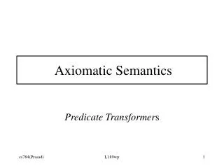
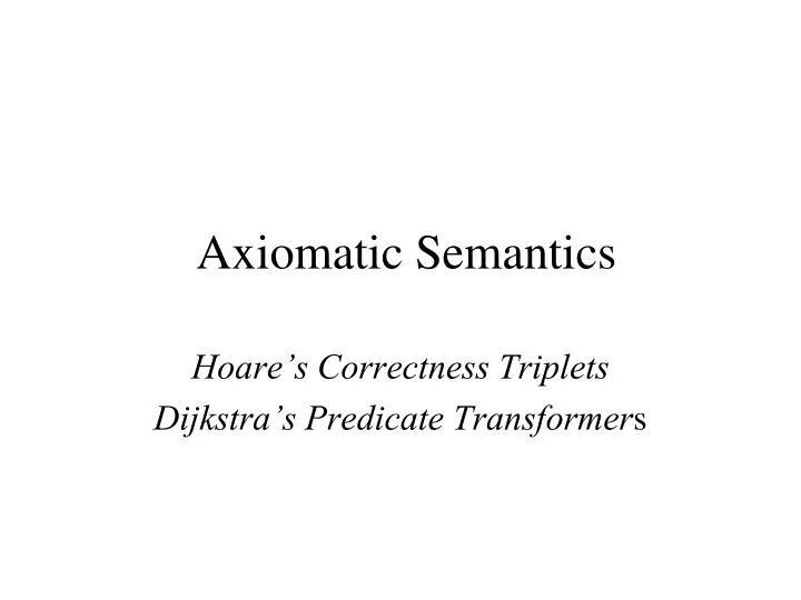
Axiomatic Semantics Hoare’s Correctness Triplets Dijkstra’s Predicate Transformers
gcd-lcm algorithm w/ invariant {PRE: (x = n) and (y = m)} u := x; v := y; while {INV: 2*m*n = x*v + y*u} (x <> y) do if x > y then x := x - y; u := u + v else y := y - x; v := v + u fi od {POST:(x = gcd(m, n)) and (lcm(m, n) = (u+v) div 2)}
Goal of a program = IO Relation • Problem Specification • Properties satisfied by the input and expected of the output (usually described using “assertions”). • E.g., Sorting problem • Input : Sequence of numbers • Output: Permutation of input that is ordered. • View Point • All other properties are ignored. • Timing behavior • Resource consumption • …
ax·i·om • n.1. A self-evident or universally recognized truth; a maxim • 2. An established rule, principle, or law. • 3. A self-evident principle or one that is accepted as true without proof as the basis for argument; a postulate. • From a dictionary
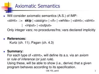
Axiomatic Semantics • Capture the semantics of the elements of the PL as axioms • Capture the semantics of composition as a rule of inference. • Apply the standard rules/logic of inference. • Consider termination separately.
States and Assertions • States: Variables mapped to Values • Includes all variables • Files etc. are considered “global” variables. • No notion of value-undefined variables • At a given moment in execution • An assertion is a logic formula involving program variables, arithmetic/boolean operations, etc. • All assertions are attached to a control point. • Assertions: States mapped to Boolean • Boolean connectives: and, or, not, implies, … • For-all, There-exists • Special predicates defined just for use in assertions (not for use in the program).
Hoare’s Logic • Hoare Triplets: {P} S {Q} • P, pre-condition assertion; S, statements of a PL; Q, post-condition assertion • If S begins executing in a state satisfying P, upon completion of S, the resulting state satisfies Q. • {P} S {Q} has no relevance if S is begun otherwise. • A Hoare triplet is either true or false. Never undefined. • The entire {P}S{Q} is considered true if the resulting state satisfies Q if and when S terminates. • If not, the entire {P}S{Q} is false.
Hoare Triplet Examples • true triplets • {x = 11 } x := 0 { x = 0 } • we can give a weaker precondition • {x = 0 } x := x + 1 { x = 1 } • {y = 0} if x <> y then x:= y fi { x = 0 } • {false } x := 0 { x = 111 } • correct because “we cannot begin” • no state satisfies false • post condition can be any thing you dream • {true} while true do od {x = 0} • true is the weakest of all predicates • correct because control never reaches post • {false} while true do od {x = 0} • false is the strongest of all predicates • false triplet • {true} if x < 0 then x:= -x fi { x > 0 }
Weaker/Stronger • An assertion R is said to be weaker than assertion P if • the truth of P implies the truth of R • written: P→R • equivalently • not P or R. • For arbitrary A, B we have: A and B → B • This general idea is from Propositional Calculus • n > 0 is of course weaker than n = 1, but this follows from Number Theory.
Weaker/Stronger Q’ stronger Q’ Q P’ weaker P P’ P’ States States P’ Q P Q’
Partial vs Total Correctness • Are P and S such that termination is guaranteed? • S is partially correct for P and Q iff whenever the execution terminates, the resulting state satisfies Q. • S is totally correct for P and Q iff the execution is guaranteed to terminate, and the resulting state satisfies Q.
Hoare Triplet Examples • Totally correct (hence, partially correct) • {x = 11} x := 0 {x = 0} • {x = 0} x := x + 1 {x = 1} • {y = 0}if x <> y then x:= y fi {x = 0} • {false} while true do S od {x = 0} • {false} x := 0 {x = 111} • Not totally correct, but partially correct • {true} while true do S od {x = 0} • Not partially correct • {true} if x < 0 then x:= -x fi {x > 0}
Assignment axiom • {Q(e)} x := e {Q(x)} • Q(x) has free occurrences of x. • Q(e): every free x in Q replaced with e • Assumption: e has no side effects. • Caveats • If x is not a “whole” variable (e.g., a[2]), we need to work harder. • PL is assumed to not facilitate aliasing.
Inference Rules • Rules are written as Hypotheses: H1, H2, H3------------------------------Conclusion: C1 • Can also be stated as: • H1 and H2 and H3 implies C1 • Given H1, H2, and H3, we can conclude C1.
Soundness and Completeness • Soundness is about “validity” • Completeness is about “deducibililty” • Ideally in a formal system, we should have both. • Godel’s Incompleteness Theorem: • Cannot have both • Inference Rules ought to be sound • What we proved/ inferred/ deduced is valid • Examples of Unsound Rules • A and B and C not B • x > y implies x > y+1 (in the context of numbers) • All the rules we present from now on are sound
Rule of Consequence • Suppose: {P’} S {Q’}, P=>P’, Q’=>Q • Conclude: {P} S {Q} • Replace • precondition by a stronger one • postcondition by a weaker one
Statement Composition Rule {P} S1 {R}, {R} S2 {Q}------------------------------{P} S1;S2 {Q} Using Rule of Consequence {P} S1 {R1}, R1 R2, {R2} S2 {Q}-----------------------------{P} S1;S2 {Q}
if-then-else-fi Hoare’s Triplets {P and B} S1 {Q} {P and not B} S2 {Q} ------------------------------------- {P} if B then S1 else S2 fi {Q} • We assumed that B is side-effect free • Execution of B does not alter state
Invariants • An invariant is an assertion whose truth-value does not change • Recall: All assertions are attached to a control point. • An Example: x > y • The values of x and y may or may not change each time control reaches that point. • But suppose the > relationship remains true. • Then x > y is an invariant
Loop Invariants • Semantics of while-loop {I and B} S {I} ------------------------------------------- {I} while B do S od {I and not B} • Termination of while-loop is not included in the above. • We assumed that B is side-effect free.
Data Invariants • Well-defined OOP classes • Public methods ought to have a pre- and post-conditions defined • There is a common portion across all public methods • That common portion is known as thedata invariant of the class.
while-loop: Hoare’s Approach • Wish to prove: {P} while B do S od {Q} • Given: P, B, S and Q • Not given: a loop invariant I • The I is expected to be true just before testing B • To prove {P} while B do S od {Q}, discover a strong enough loop invariant I so that • P => I • {I and B} S {I} • I and not B => Q • We used the Rule of Consequence twice
A while-loop example { n > 0 and x = 1 and y = 1} while (n > y) doy := y + 1; x := x*y od {x = n!}
while-loop: Choose the Invariant • Invariant I should be such that • I and not B Q • I and not (n > y) (x = n!) • Choose (n ≥ y and x = y!) as our I • Precondition Invariant • n > 0 and x=1 and y=1 n ≥ 1 and 1=1!
while-loop: Verify Invariant • I === n ≥ y and x = y! • Verify: {I and n > y} y:= y + 1; x:=x*y {I} • {I and n > y} y:= y + 1 {n ≥ y and x*y = y!} • {I and n > y} y:= y + 1 {n ≥ y and x= (y-1)!} • (I and n > y) (n ≥ y+1 and x= (y+1-1)!) • (I and n > y) (n > y and x= y!) • (n ≥ y and x = y! and n > y) (n > y and x= y!) • QED
while-loop: I and not B Q • I === n ≥ y and x = y! • n ≥ y and x = y! and not (n > y) x = n! • n = y and x = y! x = n! • QED
while-loop: Termination • Termination is not part of Hoare’s Triplets • General technique: • Find a quantity that decreases in every iteration. • And, has a lower bound • The quantity may or may not be computed by the algorithm • For our example: Consider n – y • values of y: 1, 2, …, n-1, n • values of n - y: n-1, n-2, …, 1, 0
Weakest Preconditions • We want to determine minimally what must be true immediately before executing S so that • assertion Q is true after S terminates. • S is guaranteed to terminate • The Weakest-Precondition of S is a mathematical function mapping any post condition Q to the "weakest" precondition Pw. • Pw is a condition on the initial state ensuring that execution of S terminates in a final state satisfying R. • Among all such conditions Pw is the weakest • wp(S, Q) = Pw
Dijkstra’s wp(S, Q) • Let Pw = wp(S, Q) • Def of wp(S, Q): Weakest precondition such that if S is started in a state satisfying Pw, S is guaranteed to terminate and Q holds in the resulting state. • Consider all predicates Pi so that {Pi}S{Q}. • Discard any Pi that does not guarantee termination of S. • Among the Pi remaining, choose the weakest. This is Pw. • {P} S {Q} versus P => wp(S, Q) • {Pw} S {Q} is true. • But, the semantics of {Pw} S {Q} does not include termination. • If P => wp(S, Q) then {P}S{Q} also, and furthermore S terminates.
Properties of wp • Law of the Excluded Miraclewp(S, false) = false • Distributivity of Conjunctionwp(S, P and Q) = wp(S,P) and wp(S,Q) • Law of Monotonicity(Q→R) → (wp(S,Q)→wp(S,R)) • Distributivity of Disjunctionwp(S,P) or wp(S, Q) → wp(S,P or Q)
Predicate Transformers • Assignment wp(x := e, Q(x)) = Q(e) • Composition wp(S1;S2, Q) = wp(S1, wp(S2,Q))
A Correctness Proof • {x=0 and y=0} x:=x+1;y:=y+1 {x = y} • wp(x:=x+1;y:=y+1, x = y) • wp(x:=x+1, wp(y:=y+1, x = y)) === wp(x:=x+1, x = y+1) === x+1 = y+1 === x = y • x = 0 and y = 0 x = y
if-then-else-fi in Dijkstra’swp wp(if B then S1 else S2 fi, Q) ===(B wp(S1,Q)) and(not B wp(S2,Q)) ===(B and wp(S1,Q))or(not B and wp(S2,Q))
wp-semantics of while-loops • DO == while B do S od • IF == if B then S fi • Let k stand for the number of iterations of S • Clearly, k >= 0 • If k > 0, while B do S od is the same as: • if B then S fi; while B do S od
while-loop: wp Approach • wp(DO, Q) = P0 or there-exists k > 0: Pk • States satisfying Pi cause i-iterations of while-loop before halting in a state in Q. • Pi defined inductively • P0 = not B and Q • …
wp(DO, Q) • There exists a k, k ≥ 0, such that H(k, Q) • H is defined as follows • H(0, Q) = not B and Q • H(k, Q) = H(0, Q) or wp(IF, H(k-1, Q))
Example (same as before) { n>0 and x=1 and y=1} while (n > y) doy := y + 1; x := x*y od {x = n!}
Example: while-loop correctness Pre === n>0 and x=1 and y=1 P0 === y >= n and x = n! Pk === B and wp(S, Pk-1) P1 === y > n and y+1>=n and x*(y+1) = n! Pk === y=n-k and x=(n-k)! Weakest Precondition: W === there exists k >= 0 such that P0 or Pk Verification : For k = n-1: Pre => W
Induction Proof • Hypothesis : Pk = (y=n-k and x=(n-k)!) • Pk+1 = B and wp(S,Pk) • = y<n and (y+1 = n-k) and (x*(y+1)=(n-k)!) • = y<n and (y = n-k-1) and (x = (n-k-1)!) • = y<n and (y = n- k+1) and (x = (n- k+1)!) • = (y = n - k+1) and (x = (n - k+1)!) • Examples of Valid preconditions: • { n = 4 and y = 2 and x = 2 } (k = 2) • { n = 5 and x = 5! and y = 6} (no iteration)
Detailed Work wp(y:=y+1;x:=x*y, x=y!and n>=y) = wp(y:=y+1, x*y=y! and n>=y) = wp(y:=y+1, x=(y-1)! and n>=y) = x=(y+1-1)! and n>=y+1) = x=y! and n>y
gcd-lcm algorithm w/ invariant {PRE: (x = n) and (y = m)} u := x; v := y; while {INV: 2*m*n = x*v + y*u} (x <> y) do if x > y then x := x - y; u := u + v else y := y - x; v := v + u fi od {POST:(x = gcd(m, n)) and (lcm(m, n) = (u+v) div 2)}
gcd-lcm algorithm proof • PRE implies Loop Invariant • (x = n) and (y = m) implies 2*m*n = x*v + y*u • {Invariant and B} Loop-Body {Invariant} {2*n*m = x*v + y*u and x <> y}loop-body{2*n*m = x*v + y*u} • Invariant and not B implies POST 2*n*m = x*v + y*u and x == yimplies(x = gcd(n,m)) and (lcm(n,m) = (u+v) div 2)
gcd-lcm algorithm proof • Invariant and not B implies POST 2*m*n = x*v + y*u and x == yimplies(x = gcd(m, n)) and (lcm(m, n) = (u+v) div 2) • Simplifying 2*m*n = x*(u + v) and x == yimplies(x = gcd(m, n)) and (lcm(m, n) = (u+v) div 2)
gcd-lcm algorithm proof • Simplifying 2*m*n = x*(u + v) and x == yimplies(x = gcd(m, n)) and (x*lcm(m, n) = m*n) • Simplifying 2*m*n = x*(u + v) and x == yimplies(x = gcd(m, n)) and (x*lcm(m, n) = m*n)
Some Properties of lcm-gcd • gcd() and lcm() are symmetric • gcd(m, n) = gcd(n, m) • lcm(m, n) = lcm(n, m) • gcd(m, n) = gcd(m + k*n, n) • where k is a natural number. • gcd(m, n) * lcm(m, n) = m * n