Download
1 / 35
350 likes | 498 Views
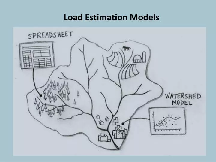
Load Estimation Models. Existing loads come from:. Point-source discharges (NPDES facilities) Info is available on the discharges (DMRs, etc.) Some are steady-flow, others are precip-driven Nonpoint sources All are (mostly) precipitation-driven

E N D
Existing loads come from: • Point-source discharges (NPDES facilities) • Info is available on the discharges (DMRs, etc.) • Some are steady-flow, others are precip-driven • Nonpoint sources • All are (mostly) precipitation-driven • Calculating the “wash-off, runoff” load is tough • Literature values can be used to estimate • Modeling gets you closer . . . . do you need it? • Air/atmospheric deposition • Can be significant in some locations
Limitations of Data-driven Approaches • Monitoring data • Reflect current/historical conditions (limited use for future predictions) • Insight limited by extent of data (usually water quality data) • Often not source-specific • May reflect a small range of flow conditions • Literature • Not reflective of local conditions • Wide variation among literature • Often a “static” value (e.g., annual)
If a Data-driven Approach Isn’t Enough…Models are Available What is a Model? • A theoretical construct, • together with assignment of numerical values to model parameters, • incorporating some prior observations drawn from field and laboratory data, • and relating external inputs or forcing functions to system variable responses * Definition from: Thomann and Mueller, 1987
Nuts and Bolts of a Model Input Model Algorithms Output Factor 1 Rainfall Event System Response Land use Factor 2 Soil Pollutant Buildup Stream Pt. Source Factor 3 Others
Is a Model Necessary? It depends what you want to know… Probably Not • What are the loads associated with individual sources? • Where and when does impairment occur? • Is a particular source or multiple sources generally causing the problem? • Will management actions result in meeting water quality standards? • Which combination of management actions will most effectively meet load targets? • Will future conditions make impairments worse? • How can future growth be managed to minimize adverse impacts? Probably Models are used in many areas… TMDLs, stormwater evaluation and design, permitting, hazardous waste remediation, dredging, coastal planning, watershed management and planning, air studies
Types of Models • Landscape models • Runoff of water and materials on and through the land surface • Receiving water models • Flow of water through streams and into lakes and estuaries • Transport, deposition, and transformation in receiving waters • Watershed models • Combination of landscape and receiving water models • Site-scale models • Detailed representation of local processes, for example Best Management Practices (BMPs)
Crops Crops Pasture Pasture Urban Urban Types of Models • Landscape/Site-scale models • Receiving water models • Watershed models
Model Basis • Empirical formulations • mathematical relationship based on observed data rather than theoretical relationships • Deterministic models • mathematical models designed to produce system responses or outputs to temporal and spatial inputs (process-based)
Review of Commonly Used Models • Landscape and Watershed models • Simple models • Mid-range models • Comprehensive watershed models • Field-scale models
Simple Models • Loading Rate • Simple Method • USLE / MUSLE • USGS Regression • PLOAD • STEPL • Minimal data preparation • Landuse, soil, slope, etc. • Good for long averaging periods • Annual or seasonal budgets • No calibration • Some testing/validation is preferable • Comparison of relative magnitude Limitations: • Limited to waterbodies where loadings can be aggregated over longer averaging periods • Limited to gross loadings
Mid-range Models • AGNPS • GWLF • P8 • SWAT ( + receiving water) • More detailed data preparation • Meteorological data • Good for seasonal/event issues • Minimal or no calibration • Testing and validation preferable • Application objectives • Storm events, daily loads • Limitations: • Limited pollutants simulated • Limited in-stream simulation & comparison w/standards • Daily/monthly load summaries
Comprehensive Watershed Models • HSPF/LSPC • SWMM • Accommodate more detailed data input • Short time steps and finer configuration • Complex algorithms need state/kinetic variables • Ability to evaluate various averaging periods and frequencies • Calibration is required • Addresses a wide range of water and water quality problems • Include both landscape and receiving water simulation • Limitations: • More training and experience needed • Time-consuming (need GIS help, output analysis tools, etc.)
Source of Additional Information on Model Selection • EPA 1997, Compendium of Models for TMDL Development and Watershed Assessment. EPA841-B-97-007 • Review of loading and receiving water models • Ecological assessment techniques and models • Model selection
Key Considerations When Selecting a Model • Relevance • Representation of key land uses and processes • Pollutants of concern • Credibility • Peer-reviewed • Public domain and source code is available on request • Usability • Availability of documentation, training, and support • Availability and accessibility of data to run model • Model and user interface is reliable and tested • Utility • Able to predict range of management options considered
Example of Simple Model Application • Spreadsheet Tool for Estimating Pollutant Load (STEPL) • Employs simple algorithms to calculate nutrient and sediment loads from different land uses • Also includes estimates of load reductions that would result from the implementation of various BMPs • Data driven and highly empirical • A customized MS Excel spreadsheet model • Simple and easy to use
STEPL Users? • Basic understanding of hydrology, erosion, and pollutant loading processes • Knowledge (use and limitation) of environmental data (e.g., land use, agricultural statistics, and BMP efficiencies) • Familiarity with MS Excel and Excel Formulas
Runoff Erosion/ Sedimentation Process Sources Cropland Urban BMP Load before BMP Load after BMP Pasture Forest Feedlot Others STEP 1 STEP 2 STEP 3 STEP 4
STEPL Web Site Link to on-line Data server Link to download setup program to install STEPL program and documents Temporary URL: http://it.tetratech-ffx.com/stepl until moved to EPA server
STEPL Main Program • Run STEPL executable program to create and customize spreadsheet dynamically • Go to demonstration
STEPL Data Input • 11 input tables • 4 tables require you to change initial input values • Land use (acres of urban, cropland, pasture, forest, user defined, feedlots), % feedlot paved • Average rain, rain days, average rain/event • Number of agricultural animals (beef, dairy, swine, sheep, horse, chicken, turkey, duck) • Number of months manure applied • Number of septic systems, population per septic system, septic failure rate (%) • Number of people who discharge wastewater directly to streams, % reduction of people discharging directly to streams • USLE parameters (R, K, LS, C, P, R, K) for cropland, pasture, forest, and user-defined land use
STEPL Data Input • 7 tables contain default values that you may choose to change: • BMPs and efficiencies for N, P, BOD, and sediment on cropland, pasture, forest, user-defined land use, urban, and feedlots • % of land use area to which each BMP is applied • Combined watershed BMP efficiencies from the BMP calculator if interactions of BMPs are considered (optional)
STEPL Data Input • Optional greater detail: • Average soil hydrologic group • Soil N, P, and BOD concentrations (%) • N, P, and BOD concentrations in runoff and shallow ground water from each land use • Reference runoff curve numbers (A, B, C, D) for each land use and subcategories of urban land use • Acreage of urban subcategories (e.g., commercial, multi-family, vacant) • Cropland irrigation (acres, inches pre- and post-BMPs, times/year)
Other Features of STEPL • Lots of default values/options: • Rainfall and USLE parameters based on location and nearby weather station • BMPs can be added and efficiencies can be edited • Urban BMP Tool for BMPs or LIDs for urban land uses
Other Features of STEPL • Gully and Streambank Erosion Tool input parameters • Gully dimensions • Number of years gully has taken to form the current size • Gully stabilization (BMP) efficiency (0-1) and the gully soil textural class • Streambank dimensions • Lateral recession rate (ft/yr) of the eroding streambank • Streambank stabilization (BMP) efficiency (0-1) and streambank soil textural class
STEPL Outputs • Pollutant loads and reductions will be calculated and graphed
STEPL Output as Function of Input Data Accuracy Minor tinkering with several parameters resulted in the following ranges for P Load
STEPL Outputs • BMP Efficiencies are MAJOR driving force for load reductions and are quite insensitive to changes in other parameters (e.g., rainfall) • Need to have a very good sense of the true efficiencies in each situation (i.e., starting point is key) • Rainfall data must be accurate or loads can vary considerably (but % reduction won’t change much!)
Region 5 Load Reduction Model • Spreadsheet to estimate loads and load reductions • Gullies, bank stabilization, and agriculture fields and filter strips: • Sediment, P, and N • Feedlots: • BOD, P, and N • Urban: • BOD, COD, TSS, Pb, Cu, Zn, TDS, TKN, TN, DP, TP, and Cd Michigan DEQ, 1999
AVGWLF (www.avgwlf.psu.edu) • Facilitates use of GWLF (Generalized Watershed Loading Function) with ArcView interface • Used on TMDL projects in Pennsylvania • GWLF (Haith and Shoemaker, 1987) • Continuous simulation model • Simulates runoff, sediment, N, and P watershed loadings given variable-size source areas (e.g., agriculture, forest, and developed) • Has algorithms for calculating septic system loads, and allows for the inclusion of point source discharge data • Monthly calculations are made for sediment and nutrient loads, based on the daily water balance accumulated to monthly values
AVGWLF General Approach • Derive input data for GWLF for use in an “impaired” watershed • Simulate N, P, & sediment loads in impaired watershed • Compare simulated loads in impaired watershed vs. loads simulated for a nearby “reference” watershed (unimpaired but with similar landscape, development and agricultural patterns) • Evaluate potential mitigation strategies for impaired watershed to achieve pollutant loads (average annual nutrient and sediment loads ) similar to those calculated for the reference watershed
Conclusions • Many tools are available to quantify pollutant loads • Approach depends on intended use of predictions • Simplest approaches are data-driven • Watershed modeling is more complex and time-consuming • provides more insight into spatial and temporal characteristics • useful for future predictions and evaluation of management options • One size does NOT fit all!
References Haith, D.A. and L.L. Shoemaker, 1987. Generalized Watershed Loading Functions for Stream Flow Nutrients. Water Resources Bulletin, 23(3), pp. 471-478. Michigan DEQ. 1999. Pollutants Controlled Calculation and Documentation for Section 319 Watersheds Training Manual, Michigan Department of Environmental Quality, Surface Water Quality Division, Nonpoint Source Unit, Lansing, Michigan. http:\\www.deq.state.mi.us Thomann, R.V. and J.A. Mueller, 1987. Principles of Surface Water Quality Modeling and Control, Harper and Row, NY.