Download

1 / 37
390 likes | 586 Views
CS 552/652 Speech Recognition with Hidden Markov Models Winter 2011 Oregon Health & Science University Center for Spoken Language Understanding John-Paul Hosom Lecture 18 March 9 Acoustic-Model Strategies for Improved Performance. Next Topics: Improving Performance of an HMM.

E N D
CS 552/652 Speech Recognition with Hidden Markov Models Winter 2011 Oregon Health & Science University Center for Spoken Language Understanding John-Paul Hosom Lecture 18 March 9 Acoustic-Model Strategies forImproved Performance
Next Topics: Improving Performance of an HMM • Search Strategies for Improved Performance • Null States • Beam Search • Grammar Search • Tree Search • Token Passing • “On-Line” Processing • Balancing Insertion/Deletion Errors • Detecting Out of Vocabulary Words • Stack (A*) Search • Word Lattice or Word Graph • Grammar, Part II • WFST Overview • Acoustic-Model Strategies for Improved Performance • Semi-Continuous HMMs • State Tying / Clustering • Cloning • Pause Models • Summary: Steps in the Training Process
Next Topics: Improving Performance of an HMM • Acoustic Model: Model of state observation probabilities andstate transition probabilities (the HMM model ) formapping acoustics (observations) to words. • ( values are usually specified by what words (and phonemes within these words) can begin an utterance, and/or is otherwise ignored.) • Typically, focus of Acoustic Model is on state observation probabilities, because model of state transition probabilities is quite simple. • Language Model: Model of how words are connected to formsentences.
Semi-Continuous HMMs (SCHMMs) • HMMs require a large number of parameters: • One 3-state, context-dependent triphone with 16 mixture components and 26 features (e.g. MFCC + MFCC): • (26×2×16+16) × 3 = 2544 parameters • 45 phonemes yields 91125 triphones • 2544 × 91125 = 231,822,125 parameters for complete HMM • If MFCC features are used, then 39 features to model an observation and 345,546,000 parameters in the HMM. • If want 10 samples (frames of speech) per feature dimension and per mixture component for training acoustic model, need121.5 hours of speech assuming that all training data is distributed perfectly and evenly across all states. In practice,some triphones are very common and many are very rare. • Methods of addressing this problem: semi-continuous HMMs or state tying
Semi-Continuous HMMs (SCHMMs) • So far, we’ve been talking about continuous and discrete HMMs. • “Semi-continuous” or “tied mixture” HMM combines advantages of continuous and discrete • Instead of each state having separate GMMs, each with its own set of mixture components, a SCHMM has one GMM. All states share this GMM, but each state has different mixture weights. • no quantization error • more accurate results • slow • many parameters • quantization error • less accurate results • fast • few parameters
Semi-Continuous HMMs (SCHMMs) • Result is a continuous probability distribution but each statehas only a few parameters (mixture component weights) • Less precise control over probabilities output by each state, butmuch fewer parameters in estimation because the number ofGaussian components is independent of the number of states. • SCHMMs are more effective the more parameters can be shared; sharing can occur the more the feature space for different states overlaps. • So, SCHMMs are most effective with triphone-model HMMs (as opposed to monophone HMMs) because the region of feature space for one phoneme contains about 2000 triphone units(45 left contexts × 45 right contexts per phoneme = 2025). • SCHMMs also more effective when amount of training data is limited.
0.0 1.0 Semi-Continuous HMMs Semi-Continuous HMMs (SCHMMs) • In continuous HMMs, each GMM estimates probability of observation data given a particular state: 0.0 1.0 State A 0.0 1.0 State B • In SCHMMs, use one set of Gaussian components for all states: • This is the semi-continuous HMM “codebook.” (In real applications, means of each component are not necessarily evenly distributed across the feature space as shown here.)
0.0 1.0 Semi-Continuous HMMs (SCHMMs) • Semi-Continuous HMM then varies only the mixture component weights for each state. (The mean and covariance data remains the same for all states.) • State A has 7 parameters for bA(ot), state B has 7 parameters for bB(ot), plus including 7 sets of mean and covariance data for SCHMM codebook. 0.4 0.3 0.2 0.1 0.0 State A State B State A: c1 = 0.15, c2 = 0.39, c3 = 0.33, c4 = 0.10, c5 = 0.03, c6 = 0.00, c7=0.00 State B: c1 = 0.00, c2 = 0.05, c3 = 0.13, c4 = 0.36, c5 = 0.25, c6 = 0.12, c7=0.09
Semi-Continuous HMMs Semi-Continuous HMMs (SCHMMs) • Historically, there was a significant difference between continuous HMMs and SCHMMs, but more recently continuous HMMs use large amount of state tying, so advantage of SCHMMs is reduced. • SPHINX-2 (CMU) is most well-known SCHMM (and has accuracy levels approximately as good as other (continuous) HMMs) • SPHINX-3 and higher versions use tied GMMs instead • Number of parameters for SCHMM: • (number of parameters per Gaussian component • number of mixture components) + • (number of states number of mixture components) • is usually less than number of parameters for continuous HMM,and almost always less if don’t store unnecessary (zero) values.
Semi-Continuous HMMs Semi-Continuous HMMs (SCHMMs) • For example, 3-state, context-dependent triphone SCHMM with 1024 mixture components and 26 features (e.g. MFCC + MFCC): • ((26×2×1024) + (91125×1024)) = 93,365,248 parameters • or about half the number of parameters of a comparable continuous HMM. • If we only store about 16 non-zero components per state along with information about which state is non-zero (again comparable to continuous HMM), then • ((26×2×1024) + (91125×16×2)) = 3,022,496 parameters • or about 1% to 2% the size of a comparable continuous HMM • Fewer number of parameters for modeling the same amount of data can yield more accurate acoustic models if done properly.
Semi-Continuous HMMs (SCHMMs) • Advantages of SCHMMs: • Minimizes information lost due to VQ quantization • Reduces number of parameters because probability density functions are shared • Allows compromise for amount of detail in model based on amount of available training data • Can jointly optimize both codebook and other HMM parameters (as with discrete or continuous HMMs) usingExpectation Maximization • Fewer number of parameters yields faster operation (which can, in turn, be used to increase the beam width during Viterbi search for improved accuracy instead of faster operation).
/s-ae+k/ 1 /k-ae+t/ 1 /s-ae+t/ 1 /s-ae+k/ 2 /k-ae+t/ 2 /s-ae+t/ 2 /s-ae+k/ 3 /k-ae+t/ 3 /s-ae+t/ 3 State Tying/Clustering • State Tying: Another method of reducing number of parameters in an HMM • Idea: If two states represent very similar data (GMM parametersare similar) then replace these two states with a single stateby “tying” them together. • Illustration with 3-state context-dependent triphones: /s-ae+t/ /k-ae+t/ /s-ae+k/ tie these 2 states tie these 2 states
State Tying/Clustering • “Similar” parameters then become the same parameters, sodecreases ability of HMM to model different states. • Can tie more than 2 states together. • “Logical” model still has 45 × 45 × 45 = 91125 triphones. But“physical” model has fewer parameters (M× 45 ×N, whereM and N are both less than 45) • Multiple “logical” states map to single “physical” state • The question is then which states to tie together? When are two or more states “similar” enough to tie? If states are tied, will HMM performance increase (because of more parameters for estimating model parameters) or decrease (because of reduced ability to distinguish between different states)?
State Tying/Clustering • Tying can be performed at multiple levels… • But typically we’re most interested in tying states (or, morespecifically, GMM parameters) • The process of grouping states (or other levels of information) together for tying is called clustering. HMM state aij GMM components jkjkcjk
State Tying/Clustering • How to decide which states to tie? Clustering algorithm • Method 1: • Knowledge-Based Clustering • e.g. tie all states of /g-ae+t/ to /k-ae+t/ because (a) not enoughdata to robustly estimate /g-ae+t/ and (b) /g/ is acousticallysimilar to /k/. • e.g. tie /s-ih-p/ state 1 to /s-ih-k/ state 1 (same left context) • Method 2: • Data-Driven Clustering • Use distance metric to merge “close” states together • Method 3: • Decision-Tree Clustering • Combines knowledge-based and data-driven clustering
State Tying/Clustering: Data-Driven Clustering • Given: • all states initially having individual clusters of data • a distance metric between clusters A and B • (weighted) distance between the means • Kullback-Liebler distance • measure of cluster size • e.g. largest distance between points X and Y in cluster • thresholds for largest cluster size, minimum number of clusters • Algorithm: • (1) Find pair of clusters A and B with minimum (but non-zero) cluster distance • (2) Combine A and B into one cluster • (3) Tie all states in A with all states in B, creating 1 new cluster • (4) Repeat from (1) until thresholds reached • Optional: (5) while any cluster has less than a minimum number of data points, merge that cluster with nearest cluster
State Tying/Clustering: Data-Driven Clustering • Distance Metrics: • (Weighted) Euclidean Distance Between Means(D=dimension of feature space, x and y are two clusters) • Euclidean Distance Weighted Euclidean Distance • between the means or Mahalanobis Distance • Symmetric Kullback-Liebler Distance(i = data point in training data set I)
State Tying/Clustering: Data-Driven Clustering Example with 1-dimensional, weighted Euclidean distance, where MX,Y is the distance between two clusters X and Y: cluster1 cluster2 cluster3 cluster4 0.10 0.40 0.60 0.95 0.15 0.30 0.65 0.80 0.05 0.45 0.50 0.95 0.10 0.30 0.70 0.85 mean= 0.10 0.36 0.61 0.89 st.dev.= 0.0408 0.075 0.0854 0.075 M1,1=0.0 M1,2=4.70 M1,3=8.64 M1,4=14.28 M2,2=0.0 M2,3=3.12M2,4=7.07 M3,3=0.0 M3,4=3.50 M4,4=0.0 So we group clusters 2 and 3. data points in cluster
State Tying/Clustering: Data-Driven Clustering Example, continued… cluster1 cluster 2,3 cluster 4 0.10 0.40, 0.60 0.95 0.15 0.30, 0.65 0.80 0.05 0.45, 0.50 0.95 0.10 0.30, 0.70 0.85 mean= 0.10 0.49 0.89 st.dev.= 0.0408 0.1529 0.075 M1,1=0.0 M1,23=4.94 M1,4=14.28 M23,23=0.0 M23,4=3.73 M4,4=0.0 So we group clusters (2,3) and 4.
State Tying/Clustering: Decision-Tree Clustering* • What is a Decision Tree? • Automatic technique to cluster similar data based on knowledge of the problem • (combines data-driven and knowledge-based methods) • Three components in creating a decision tree: • 1. Set of binary splitting questions • Ways in which data can be divided into two groups based on knowledge of the problem • 2. Goodness-of-split criterion If data is divided into two groups based on a binary splitting question, how good is a model based on these two new groups as opposed to the original group? • 3. Stop-splitting criterion when to stop splitting process *Notes based in part from Zhao et al 1999 ISIP tutorial
State Tying/Clustering: Decision-Tree Clustering • Problem with data-driven clustering: If there’s no data for • a given context-dependent triphone state, it can’t be merged with other states using a data-driven approach… we often need to be able to tie a state with no training data to “similar” states. • Decision-Tree Clustering: • Given: • a set of phonetic-based questions that provides complete coverage of all possible states.Examples: • Is left-context phoneme a fricative? • Is right-context phoneme an alveolar stop? • Is right-context phoneme a stop? • Is left-context phoneme a vowel? • the likelihood of the model given pooled set of tied states, assuming a single mixture component for each state.
State Tying/Clustering: Decision-Tree Clustering The expected value of the log-likelihood of a (single-Gaussian) leaf node (S) in the tree, given observations O=(o1,o2,…oT), is computed by the log probability of ot given this node, weighted by the probability of being in this leaf node, and summed over all times t. (Note similarity to Lecture 12, slide 11) where s = a state in the leaf node S which contains a set of tied states, t(s) = probability of being in state s at time t (from Lecture 11 Slide 6). The sum of all values is the probability of being in the tied state at time t, which is defined as having a single mixture component, with mean and covariance matrix . The log probability of a multi-dimensional Gaussian is where n is the dimension of the feature space. transpose
State Tying/Clustering: Decision-Tree Clustering It can be shown (e.g. Zhao et al., 1999) that and so the log likelihood can be expressed as and the covariance matrix of the tied state can be computed as where s and s are the mean and covariance of state s. or
State Tying/Clustering: Decision-Tree Clustering Therefore, if we have a node N that is split into two sub-nodes X and Y based on a question, the increase in likelihood obtained by splitting the node can be calculated as where LN is the likelihood of node N, LX is the likelihood of sub-node X, and LY is the likelihood of sub-node Y. The term can be computed once and stored for each state. Then, note that the increase in log-likelihood depends only on theparameters of the Gaussian states within the nodes and the values for states within the nodes, not on actual observations ot. So, computation of the increase in likelihood can be done quickly. Intuitively, the likelihood of the two-node model will be at least as good as the likelihood of the single-node model, because there are more parameters in the two-node model (i.e. two Gaussians instead of one) that are modeling the same data.
State Tying/Clustering: Decision-Tree Clustering Algorithm: 1. start with all states contained in root node of tree 2. Find the binary question that maximizes the increase in the likelihood of the data being generated by the model. 3. split the data into two parts, one part for the “yes” answer, one part for the “no” answer. 4. For both of the new clusters, go to step (2), until the increase in likelihood of data falls below threshold. 5. For all leaf nodes, compute log-likelihood of merging with another leaf node. If decrease in likelihood is less than some other threshold, then merge the leaf nodes. Note that this process models each cluster (group of states) with a single Gaussian, whereas the final HMM will model each cluster with a GMM. This discrepancy is tolerated because using a single Gaussian in clustering allows fast evaluation of cluster likelihoods.
State Tying/Clustering: Decision-Tree Clustering Illustration: s-ih+t s-ih+d s-ih+n f-ih+d f-ih+n f-ih+t d-ih+t d-ih+d d-ih+n this question was the one yielding highest likelihood is left context a fricative? N Y s-ih+t s-ih+d s-ih+n d-ih+t d-ih+d d-ih+n f-ih+t f-ih+d f-ih+n (no question causes sufficient increase in likelihood) is right context a nasal? N Y s-ih+t s-ih+d s-ih+n f-ih+t f-ih+d f-ih+n
State Cloning The number of parameters in an HMM can still be very large, even with state tying and/or SCHMMs. Instead of reducing number of parameters, another approach to training a successful HMM is to improve initial estimates before embedded training. Cloning is used to create triphones from monophones. Given: a monophone HMM (context independent) that has good parameter estimates Step 1: “Clone” all monophones, creating triphones with parameters equal to monophone HMMs. Step 2: Train all triphones using embedded training.
State Cloning Example: ih ih ih 45 cloning s-ih+t s-ih+t s-ih+t 90,000 f-ih+n f-ih+n f-ih+n f-ih+t f-ih+t f-ih+t then train all of these models using forward-backward and embedded training; then cluster similar models
Pause Models The pause between words can be considered as one of two types: long (silence) and short (short pause). The short- pause model can skip the silence-generating state entirely, or emit a small number of silence observations. The silence model allows transitions from the final silence state back to the initial silence state, so that long-duration silences can be generated. 0.2 states are tied 0.3 (Figure from Young et. al, The HTK Book)
Pause Models • The pause model is trained by • initially training a 3-state model for silence • creating the short-pause model and tying its parameter values to the middle state of silence • adding transition probability of 0.2 from states 2 to 4 of state silence (other transitions are re-scaled to sum to 1.0) • adding transition probability of 0.2 from states 4 to 2 of state silence • adding transition probability of 0.3 from states 1 to 1 of the short pause state • re-training with embedded training
Steps In the Training Process • Steps in HMM Training: • Get initial segmentation of data(flat start, hand labeled data, forced alignment) • Train single-component monophone HMMs using forward-backward training on individual phonemes • Train monophone HMMs with embedded training • Create triphones from monophones by cloning • Train triphone models using forward-backward training • Tie states using decision tree • Double number of mixture components using VQ • Train with embedded training • Repeat steps (7) and (8) until get desired number of components
Steps In the Training Process train initial monophone models cloning to createtriphones; do embedded training tie states based ondecision tree clustering double number of mixture components; do embedded training (Figure from Young, Odell, Woodland, 1994)
Evaluation of System Performance • Accuracy is measured based on three components: • word substitution, insertion, and deletion errors • accuracy = 100 – (sub% + ins% + del%) • error = (sub% + ins% + del%) • Correctness only measures substitution and deletion errors • correctness = 100 – (sub % + del %) • insertion errors not counted… not a realistic measure • Improvement in a system is commonly measured using relative reduction in error: • where errorold is the error of the “old” (or baseline) system, • and errornew is the error of the “new” (or proposed) system.
State of the Art • State-of-the-art performance depends on the task… • Broadcast News in English: ~90% • Broadcast News in Mandarin Chinese or Arabic: ~80% • Phoneme recognition (microphone speech): 74% to 76% • Connected digit recognition (microphone speech): 99%+ • Connected digit recognition (telephone speech): 98%+ • Speaker-specific continuous-speech recognition systems: (Naturally Speaking, Via Voice): 95-98% • How good is “good enough”? At what point is “state-of-the-art” performance sufficient for real-world applications?
State of the Art • A number of DARPA-sponsored competitions over the years has led to decreasing error rates on increasingly difficult problems 100% Conversational Speech (Switchboard) Meeting Speech (single mic) Read Speech Switchboard II Switchboard Cellular Meeting Speech (multiple mics) Structured Speech Meeting Speech (headmounted mic) Broadcast Speech 20k Air Travel Planning (2-3k) 19% News Mandarin Varied Microphones News Arabic Noisy Speech CTS Fisher Word Error Rate (log scale) News English 1x 10% 5k News English 10x Noisy 1k human transcription of Broadcast Speech (0.9%WER) human transcription of conversational Speech (2%-4% WER) 2.5% 1988 1989 1990 1991 1992 1993 1994 1995 1996 1997 1998 1999 2000 2001 2002 2003 2004 2005 2006 2007 2008 2009 1% (from “The Rich Transcription 2009 Speech-to-Text (STT) and Speaker-Attributed STT (SASTT) Results” (Ajot & Fiscus))
State of the Art • We can compare human performance against machine performance (best results for machine performance): • Task Machine Error Human Error • Digits 0.72% 0.009% (80) • Letters 9.0% 1.6% (6) • Transactions 3.6% 0.10% (36) • Dictation 7.2% 0.9% (8) • News Transcription 10% 0.9% (11) • Conversational Telephone Speech 19% 2%-4% (5 to 10) • Meeting Speech 40% 2%-4% (10 to 20) • Approximately an order of magnitude difference in performance for systems that have been developed for these particular tasks/environments… performance worse for noisy and mismatched conditions • Lippmann, R., “Speech Recognition by Machines and Humans,” Speech Communication, vol. 22, no. 1, 1997, pp. 1-15.
Why Are HMMs Dominant Technique for ASR? • Well-defined mathematical structure • Does not require expert knowledge about speech signal (more people study statistics than study speech) • Errors in analysis don’t propagate and accumulate • Does not require prior segmentation • Temporal property of speech is accounted for • Does not require a prohibitively large number of templates • Results are usually the best or among the best