Download
1 / 7
70 likes | 204 Views
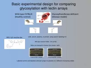
Basic experimental design for comparing glycosylation with lectin arrays. Wild-type C57BL/ 6 (Healthy control) . Glycosyltransferase deficient (Disease model). cells, serum, plasma, or protein prep used in labeling rxn. NHS -Cy5 reactive dye.

E N D
Basic experimental design for comparing glycosylation with lectin arrays Wild-type C57BL/6 (Healthy control) Glycosyltransferase deficient (Disease model) cells, serum, plasma, or protein prep used in labeling rxn NHS -Cy5 reactive dye NHS dye reaction killed (Tris pH 8) Slides are clamped in frames that creates wells Incoming slide sample Control slide sample Labeled control and labeled unknown preps incubated on 2 different microarray slides
1st slide, a control, 12 subgrids, triplicate read averaged, H/L calculated for each lectin High and low for each lectin become the boundaries for no change High Value H6 H5 H4 H3 H2 No change region H1 L1 L2 L3 L4 L5 Low value L6
A second slide, an unknown or incoming sample, 12 subgrids, triplicate read averaged, median calculated for each lectin H6 H5 H4 Median calculated H3 H2 Less sensitive to outliers H1 A AMA L1 L2 L3 L4 L5 L6
Comparison of unknown median read to control high and low boundary Above boundary, digitization = 1 Control high value boundary H6 Control Within boundaries, digitization = 0 No change region Control low value boundary Below boundary, digitization = -1 L6
Confidence assignments for digitization =0 • For each lectin in the unknown which has a 0 digitization value, a confidence factor is assigned based on its position relative to the control high low range • median value for the unknown is placed within a bin in the L/H control range • the distance from the mid point of the control range sets the bin # (certainty level) For digitization = 0 -0 confidence border +0 confidence border Confidence=1 Bin 1 Bin -10 Bin 10 Bin 8 Bin -5 Bin -1 Midpoint of H/L Ex#2: Median value of unknown (bin 8) +0.8 confidence Ex#1: Median value of unknown (bin -1) -0.1 confidence • A bin # of -1 or 1 is near the high or the low control boundaries • has a small percentage confidence value • has a negative or positive value depending on position relative to mid point L6 H6
Confidence assignments for digitization = -1 and +1 • For each lectin in the unknown which has a -1 or +1 digitization value • a confidence factor is assigned based on its signal position relative to: • either thecontrol low boundary orcontrol high boundary digitization = 1 area Control range midpoint Low boundary High boundary A B Point A would have a better confidence factor then B: i.e.- less relative signal digitization = -1 area
Example calculation of the confidence level for a digitization = -1 500 RFU (LB-control Low Boundary value) 1000 RFU Incoming value point (DS) (HB-control High Boundary) Control H/L range • Large decrease, in relation to large value low boundary, gives high confidence • similarly • Small decrease in relation to a small value low boundary gives a high confidence DS- Incoming Decreased Signal Relative Fluoresence Units Confidence factor= (DS-LB)/DS EX. 500 – 1000 /500 = -1 confidence factor (a 50% decrease in signal)