Download
1 / 24
240 likes | 409 Views
Meeting Forest Carbon Planning Needs with Forest Service Data and Satellite Imagery. Sean Healey, Gretchen Moisen RMRS Inventory, Monitoring, and Analysis Program. Todd Morgan U. MT Bureau of Business and Economic Research. Greg Jones, Dan Loeffler RMRS Human Dimensions Program.

E N D
Meeting Forest Carbon Planning Needs with Forest Service Data and Satellite Imagery Sean Healey, Gretchen Moisen RMRS Inventory, Monitoring, and Analysis Program Todd Morgan U. MT Bureau of Business and Economic Research Greg Jones, Dan Loeffler RMRS Human Dimensions Program Shawn Urbanski RMRS Fire, Fuel, and Smoke Program Jim Morrison, Barry Bollenbacher, Renate Bush, Keith Stockman National Forest System, Region 1
Montana Idaho The Forest Carbon Management Framework (ForCaMF) has been piloted in Ravalli County, MT, and is currently being applied across the NFS Northern region
Managers and planners need comprehensive information about carbon stocks and flows • Big Picture: How much carbon is the landscape storing or emitting? • What are the immediate and long-term effects of natural disturbance on carbon storage? • How does carbon accumulation in undisturbed parts of the landscape compare with disturbance losses? • What is the magnitude of harvest effects vs. “natural processes”?
The Forest Service maintains a stand dynamics tool (Forest Vegetation Simulator - FVS) that is used in ForCaMF to govern carbon accumulation and emission across the landscape.
Estimation of ecosystem flux Starting Point Ravalli County (MT) forest volume, 1985 • Mid-1980s imagery is used spatially represent FIA estimates from the same era. The landscape matches FIA in the following ways: • Area of forest • Area of forest by forest type • Mean volume • Distribution of volume (right number of low-, medium-, and high-volume pixels) 50 km
Estimation of ecosystem flux Starting Point • Spatial representations of reference data are prepared using satellite imagery Forest Type Disturbance 1985 Forest Volume Fir, Spruce Lodgepole No disturbance Burn Greyscale: low to high Non-forest Non-forest/ Background Cut Doug Fir Ponderosa
1985 Carbon FVS-derived carbon dynamics are applied according to the spatial inputs to create the best available spatial representation of carbon sequestration over time 1985 Forest Volume 1987 Carbon Forest Type 1989 Carbon 1985 Carbon Disturbance However, we know that there is uncertainty involved with each of the inputs … 1985 Carbon
Plot-Level Model Calibration Plot-Level Basis for Simulation Inventory Data FVS Carbon Simulations Forest Type Population-Level Model Constraint Forest Volume Probabilistic Treatment of Spatial Inputs (PTSI) Starting-Point Forest Condition Maps Lookup tables linking the starting landscape variables and disturbance history of each SU with appropriate FVS carbon simulations Spatial inputs of each SU are altered probabilistically to represent their random error and potential bias + 10-ha Simulation Units (SU) are developed representing homogeneous groupings of pixels with identical combinations of starting conditions and disturbance parameters Stocks and fluxes estimated within and summed across Simulation Units Disturbance Type % Cover Loss ENDPOINT: Probability Density Function of Stock or Flux of interest Volume harvested Spatial disturbance data
Probability Density Function (PDF) • Used in ForCaMF to describe and simulate uncertainty of inputs due to random error and bias as well as uncertainty • Also used to describe ForCaMF outputs Figure from wikipedia.org
Uncertainty built into the simulations is estimated from the best available sources, including FIA
Inputs, such as disturbance history, may be changed to derive estimates for alternative scenarios Bars represent standard deviation of 2000 simulations
Unlike standard FIA carbon stock estimates, we can isolate individual processes contributing to overall carbon flux 1.9 million (±.4 million) Average Annual Fossil Fuel Emissions Bars indicate standard deviation of 2000 simulations
We see that the net effect of fire on carbon stores actually increases for decades after the fire Estimated stand carbon in forest population affected by fire in the year 2000 in Ravalli County, MT Tonnes Carbon
Preliminary programming has occurred to embed PTSI in a decision support tool for the NFS Northern Region
Framework For each time period, PTSI-based ecosystem flux estimates may be combined with non-ecosystem flux estimates Sequestration Growth – undisturbed forests Growth – recovering forests Landscape Carbon Exchange (tonnes C) Fossil fuel combustion – road building Time Fossil fuel combustion – timber haul Combustion emissions Net of all considered factors Emission
The basic function of the system is to monitor (with uncertainty estimates) forest carbon flux over time. Alternative scenarios will be discussed later. Sequestration Landscape Carbon Exchange (tonnes C) Time Emission
Haul distances can be translated to fossil fuel emissions associated with timber transport Transport emissions for Ravalli County timber From: Healey and others, Carbon Balance and Management 4:9.
We can also estimate carbon emissions related to forest road-building over time Source: Loeffler, Jones, Vonessen, Healey, Chung. 2008. Estimating Diesel Fuel Consumption and Carbon Dioxide Emissions from Forest Road Construction. In: Forest Inventory and Analysis (FIA) Symposium; October 21-23, 2008; Park City, UT. Proc. RMRS-P-56CD.
Using dynamics in the forest product life cycle literature with harvest records, we can track emissions from historically harvested timber • More on this method: Healey et al., 2008: http://www.treesearch.fs.fed.us/pubs/33355
Flux Diagnosis Sequestration Growth – undisturbed forests Growth – recovering forests Landscape Carbon Exchange (tonnes C) Fossil fuel combustion – road building Time Fossil fuel combustion – timber haul Combustion emissions Net of all considered factors Emission
Sequestration Landscape Carbon Exchange (tonnes C) Time Emission
Alternative disturbance scenarios drive different flux trends Landscape Carbon Exchange (tonnes C) Time
Summary • Probabilistic treatment of spatial inputs (PTSI) allows us to link satellite and inventory data with FVS to understand landscape carbon dynamics and associated uncertainties • We can combine ecosystem and non-ecosystem fluxes to comprehensively track effects of disturbance and management on forest carbon storage, using both observed and hypothetical scenarios
Questions? Sean Healey seanhealey@fs.fed.us, 801-625-5770