Download
1 / 23
230 likes | 361 Views
Using the Sunyaev-Zeldovich Effect to Determine H o and the Baryon Fraction. by Michael McElwain Astronomy 278: Anisotropy and Large Scale Structure in the Universe Instructor: Edward L. Wright. Overview. Qualitative explanation of the Sunyaev-Zel’dovich Effect (SZE)

E N D
Using the Sunyaev-Zeldovich Effect to Determine Ho and the Baryon Fraction by Michael McElwain Astronomy 278: Anisotropy and Large Scale Structure in the Universe Instructor: Edward L. Wright
Overview • Qualitative explanation of the Sunyaev-Zel’dovich Effect (SZE) • Brief quantitative explanation of the SZE • Instruments employed and observations • Current Results
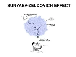
The Sunyaev-Zel’dovich Effect X-ray image of Abell 262 • First predicted by the Russian scientists Sunyaev and Zel’dovich in 1969. • Galaxy Clusters have hot gas • Tgas~10-100 million Kelvin • Electron scattering from nuclei produces X-rays, thermal bremsstahlung. • Compton scattering occurs between CMB photons and the hot electrons. • ~1% of CMB photons will interact with the hot electrons • Energy will be transferred from the hot electrons to the low energy CMB photons, changing the shape of their intensity vs. frequency plot. • Measurements made at low frequencies will have a lower intensity, since photons which originally had these energies were scattered to higher energies. This distorts the spectrum by ~0.1%. • Estimates of cosmological parameters (ie. Ho and b) can be made by combining these measurements. SZE Image of MS 1054 Mohr
Sunyaev-Zeldovich effect 0 Kompaneets equation: how the radiation changes with diffusion n/ y = 1/xe2 * / xe * xe4 *(n/ xe + n + n2), where xe = h/kBTe and y is the Compton y-parameter, y = neTkBTe/(mec2) dl variables defined: ne = number density of the electron gas Te = temperature of the electron gas T = Thompson cross-section for scattering assumptions 1. Tgas is much hotter than Trad 2. CMB radiation behaves as a blackbody 3. each photon will only scatter once Birkinshaw
Measured Quantities • Cluster redshift, z • Temperature decrement through the center of the galaxy, T • Angular diameter of the cluster, d • X-ray flux from the center of the cluster, bx • Temperature of the electron gas, Te • Temperature of the CMB
Measuring the CMB Decrement from a Cluster • Consider simplest model of cluster • Spherical with radius R • Constant gas number density n • Constant temperature Te • Sunyaev-Zel’dovich Effect decrement T • Directly related to the density • Directly related to the cluster path length • Directly related to the temperature of the gas, Te R n Te Temperature Decrement T = -TCMB2y or T TCMB2Rn Mohr Constant Density Gas Sphere
Measuring X-ray Emission from a Cluster Abell 2319 • Model of the cluster • Sphere of radius, R • Central number density of the electron gas, n • Temperature of the gas, Te • X-ray surface brightness bx • Directly related to square of density • Directly related to the cluster path length R X-ray brightness n Te bx 2Rn2 Constant Density Gas Sphere Mohr
Measuring the Size of a Cluster T/TCMB = 2Rn • Combined observations of bx and T measure the path length along the line of sight. • Us the radius of the cluster and the angular size to make an estimate at the cluster distance. Remember, we assumed that the cluster was spherical. bx 2Rn2 R = (T/TCMB)2/ 2*bx R q dA dA R/ Ho = v/ dA Distance independent of redshift! Mohr
Sunyaev-Zel’dovich signal • SZE distortion of the CMB signal. Note the decrement on the low frequency side, and the increment at higher frequencies. • The amplitude of the distortion is proportional to Te, although shape is independent of Te. The relativistic equation has a slightly more complicated shape. Carlstrom
Single Dish Radiometers Used to measure the SZ effect • Chibolton 25-m telescope • OVRO 40 m telescope • Plot shown to the right demonstrates one of the first detections of the SZE, a profile of CL 0016+16. Errors in single dish radiometers • atmospheric signals • Calibration by measuring the planets (6%) • Low resolution, can not subtract point sources along the line of sight of the cluster. Birkinshaw
Bolometers used to measure the SZ effect Sunyaev-Zel’dovich Infrared Experiment (SuZIE) • Observes 4 pixels simultaneously, at frequencies of 143, 217 and 350 GHz. • Three bolometers are in each pixel, which observe the same part of the sky. Therefore the atmospheric noise is correlated between each channel. • Bolometers attached to balloons are a partial solution to the atmospheric noise problem. Instruments such as PRONAOS are taking this approach. • Abell 2163 measurements taken across center of the X-ray peak, 2’10” South of the X-ray peak, and one free of sources X-ray sources. • Shows the temperature difference the bolometer will read as it scans a cluster. Birkinshaw
Interferometers Used to Measure the SZ effect: 1 Ryle Array • This 8 element array is located in Cambridge, UK, and operates at 15 GHz (2 cm.) Berkeley Illinois Maryland Association (BIMA) • This millimeter-wave array is located in Hat Creek, CA. John Carlstrom (U Chicago) and collaborators measure the SZE using the 10 antenna at 30 GHz (1cm.). Owens Valley Radio Observatory (OVRO) • This millimeter-wave array is located in Bishop, CA and run by Caltech. John Carlstrom and Steve Meyers (Caltech) use the 6, 10.4 meter antennas with 30 GHz detectors (1 cm.). ** These interferometers are only sensitive to the angular scales required to image clusters with z > 0.1
First Interferometric SZ detections • Ryle telescope, using an array of 5, 15 m., 15-GHz dishes in Cambridge. Antennae arranged to achieve the smallest baselines (100 m.). • N-S resolution is compromised because the Ryle Telescope is an E-W instrument. • This plot shows the Ryle telescope image of Cl 00016+16. Contours mark the SZE, while the gray background is the ROSAT image. Birkinshaw
BIMA/OVRO observations of the SZ effect: 2 • These data have been taken on interferometers retrofitted with 30 GHz receivers. • The array is set to small baselines, to ensure a large beam size. Carlstrom
Interferometers Used to Measure the SZ effect Cosmic Background Imager (CBI) • Located at the ALMA cite in Chajantor, Chile. These 13 antennae operate at 26-36 GHz. Degree Angular Scale Interferometer(DASI) • A sister project to the CBI, located at the South Pole. ** These interferometers are suited to measure nearby clusters.
X-ray Telescopes Used to Measure the SZ effect: 1 ROSAT • X-ray satellite in operation between 1990 and 1999. Mainly, its data has been used in conjunction with the radio observations to make estimates of Ho and b. Uncertainties of the X-ray intensity are ~ 10%. Chandra X-ray Observatory • Provides x-ray observations of the clusters to make estimates of the gas temperature. Chandra currently has the best resolution of all x-ray observatories. XMM-Newton • ESA’s X-ray telescope. Has 3 European Photon Imaging Cameras (EPIC). ** The data from Chandra and XMM-Newton should reduce the uncertainty in the X-ray intensities.
All-Sky Projects Used to Measure the SZ effect: 5 Microwave Anisotropy Probe • Measures temperature fluctuations in the CMB. Ned can tell you all about this. Planck satellite • ESA project designed to image the entire sky at CMB wavelengths. Its wide frequency coverage will be used to measure the SZ decrement and increment to the CMB photons. The expected launch date is ~2007.
Systematic Uncertainties in Current SZE Measurements • SZE calibration (8%) • X-ray calibration (10%) • Galactic absorption column density (5%) • Unresolved point sources still contaminate measurement of the temperature decrement. (16%) • Clusters that are prolate or oblate along the line of sight will be affected. A large sample of clusters should average the orientations. Or SZ method proposed from ROSAT data, in which clusters are barely resolved. (14%) • XMM/Chandra data demonstrate substructures within a cluster, known as isothermality and clumping. (20%) • Kinetic SZE (6%) Total Systematic Uncertainties: 33% Reese et al. 2001
Results of SZE Distance Measurements SZE Distance Measurements • 33 SZ distances vs. redshift Ho = 63 3 km/s/Mpc for M = 0.3 and = 0.7, fitting all SZEdistances • Results • SZE distances are direct (rather than relative) • SZE distances possible at very large lookback times • Can see the theoretical angular diameter distance relation. • High systematic uncertainties (30%) • Ho = 60 km/s/Mpc for an open M = 0.3 • Ho = 58 km/s/Mpc for a flat M = 1 Carlstrom
Measuring the Baryon Fraction ƒg ƒB = B/M then M B/ƒg B is constrained by BBN theory. Calculate ƒg by either measuring the SZE (proportional to n) or X-ray brightness (proportional to n2). Grego et al. 2001
Results of SZE Baryon Fraction Measurements • Remember, the gas mass fraction sets a lower bound for the baryon fraction. • SZ derived gas mass fraction at 65”, and extrapolate to a fiducial radius of r500(T,z), 500 times the critical mass density. • The mean gas mass fraction for 18 clusters (Grego et al.) is 0.081 + 0.009 - 0.011* h100-1
Hot gas in galaxy clusters Combined constraints from X-ray emission and SZE Direct cluster distances Baryon mass fraction Significant systematic errors, but a good theory for cosmological discriminators Conclusions
References PAPERS Birkinshaw et al. 1998 Carlstrom et al. 2000 Grego et al. 2000 Reese et al. 2001 TELESCOPES BIMA, http://bima.astro.umd.edu/ OVRO, http://www.ovro.caltech.edu/ Ryle telescope, http://www.mrao.cam.ac.uk/telescopes/ryle/ CBI, http://www.astro.caltech.edu/~tjp/CBI/ DASI, http://astro.uchicago.edu/dasi/ Chandra, http://chandra.harvard.edu/ XMM-Newton telescope, http://sci.esa.int/xmm/ ROSAT, http://heasarc.gsfc.nasa.gov/docs/rosat/rosgof.html MAP, http://map.gsfc.nasa.gov/ PLANCK, http://astro.estec.esa.nl/SA-general/Projects/Planck/ SuZIE, http://www.astro.caltech.edu/~lgg/suzie/suzie.html SuZIE observes 4 pixels on the sky simulateously at 143, 217 and 350 GHz. The three bolometers in a single photometer observe the same patch of sky at different frequencies; this atmospheric noise is well correlated between all three frequency channels. PRONAOS, http://www.cnes.fr/WEB_UK/activites/connaissance/html/Pronaos/Prons.html OTHER SITES http://astro.uchicago.edu/home/web/mohr/Compton/