Download
1 / 26
260 likes | 273 Views
A Parallel Hierarchical Solver for the Poisson Equation. http://wavelets.mit.edu/~darshan/18.337 Seung Lee Deparment of Mechanical Engineering selee@mit.edu R.Sudarshan Department of Civil and Environmental Engineering darshan@mit.edu 13 th May 2003. Outline. Introduction

E N D
A Parallel Hierarchical Solver for the Poisson Equation http://wavelets.mit.edu/~darshan/18.337 Seung Lee Deparment of Mechanical Engineering selee@mit.edu R.Sudarshan Department of Civil and Environmental Engineering darshan@mit.edu 13th May 2003
Outline • Introduction • Recap of hierarchical basis methods • Used for preconditioning and adaptivity • Implementation • Methodology • Mesh subdivision • Data Layout • Assembly and Solution • Results and Examples • Comparison with finite element discretization • Speed up with number of processors • Conclusions and Further Work
Introduction • Problem being considered: • Discretizing the operator using finite difference or finite element methods leads to stiffness matrices with large condition numbers • Need a good preconditioner (ILU, IC, circulant, domain decomp.) • Choosing such a preconditioner is “black magic” • Why create an ill-conditioned matrix and then precondition it, when you can create a well-conditioned matrix to begin with! • Instead of using: Use
Is better conditioned than Single Level Vs. Multilevel Approaches Single Level Multilevel + +
Formulation and Solution • Discretize using piecewise bilinear hierarchical bases: • Solve coarsest level problem with PCG (and diagonal preconditioning). Then determine first level details, second level details, etc • How well does this method parallelize? • Multiscale stiffness matrix is not as sparse • Are the savings over the single level method really significant? Big Question
Done by the “Oracle” Done in parallel Implementation - I: The Big Picture Read input, subdivide the mesh, and distribute node and edge info to processors For I=1:N_level*, Distribute elements Assemble K Solve system of Eqs. Use solution from previous mesh as a guess Perform inverse wavelet transform and consolidate solution No I > N_level?? Yes We (hopefully) have the converged solution!! *N_levels is known a priori
Implementation – II: Mesh Subdivision • Each parent element is subdivided into four children elements • Number of elements and DoFs increase geometrically , and the solution convergences with only a few subdivision levels Level 0 Level 1 Level 2 1 element 4 elements 16 elements
II I III IV Implementation – III: Data Layout • Degrees of freedom in the mesh are distributed linearly • Uses a naïve partitioning algorithm • Each processor gets roughly NDoF/NP dofs (the Update set) • Each processor assembles the rows of the stiffness matrix corresponding to elements in its update set • Each processor has info about all faces connected to vertices in its update set and all vertices connected to such faces • Equivalent to “basis partitioning”
Implementation – IV: Assembly and Solution • Stiffness matrices stored in the modified sparse row format • Requires less storage than CSR or CSC formats • Equations solved using Aztec • Solves linear systems in parallel • Comes with PCG with diagonal preconditioning • Inverse wavelet transform (synthesis of the final solution) • Implemented using Aztec as a parallel matrix-vector multiply
1 0 1 2 0 2 3 3 1 Input File Format 7 Number of subdivisions 4 Number of vertices 4 Number of edges 1 Number of elements 1.0 1.0 1 Coordinate (x,y) of the vertices, and boundary info -1.0 1.0 1 (i.e. 1 = constrained, 0 = free) -1.0 -1.0 1 1.0 -1.0 1 3 0 1 Edge definition (vertex1, vertex2), and boundary info 1 0 1 (i.e. 1 = constrained, 0 = free) 2 1 1 2 3 1 0 1 2 3 Element definition (edge1, edge2, edge3, edge4) Vertices Edges Elements
Results – I: Square Domain Level 1 Level 6
Single Scale vs. Hierarchical Basis Number of iterations vs. Degrees of Freedom • Same order of convergence, but fewer number of iterations for larger problems Number of Iterations Degrees of Freedom
Square Domain Solution • Coarsest mesh (level 1) – 9 DoFs, 1 iteration to solve, took 0.004 seconds on 4 procs • Finest mesh (level 6) – 4225 DoFs, 43 iteration to solve, took 0.123 seconds on 4 procs
Results – II: “L” Domain • Coarsest mesh (level 1) – 21 DoFs, 3 iteration to solve, took 0.0055 seconds on 4 procs • Finest mesh (level 6) – 12545 DoFs, 94 iteration to solve, took 0.280 seconds on 4 procs
Results – III: “MIT” Domain • Coarsest mesh (level 1) – 132 DoFs, 15 iteration to solve, took 0.012 seconds on 4 procs • Finest mesh (level 6) – 91520 DoFs, 219 iteration to solve, took 4.77 seconds on 8 procs
Single Level Vs. Hierarchical Basis Did not converge after 500 iters
Conclusions and Further Work • Hierarchical basis method parallelizes well • Provides a cheap and effective parallel preconditioner • Scales well with number of processors • With the right libraries, parallelism is easy! • With Aztec, much of the work involved writing (and debugging!) the mesh subdivision, mesh partitioning and the matrix assembly routines • Further work • Parallelize parts of the oracle (e.g. mesh subdivision) • Adaptive subdivision based on error estimation • More efficient geometry partitioning • More general element types (right now, we are restricted to rectangular four-node elements)
(Galerkin) Weak Form • Formally, • Leads to a multilevel system of equations Coarse <=> coarse interactions Coarse <=> fine interactions Fine <=> fine interactions