Download

1 / 53
540 likes | 747 Views
Segmentation-Based Stereo. Michael Bleyer LVA Stereo Vision. What happened last time?. Once again, we have looked at our energy function: We have investigated the matching cost function m (): Standard measures: Absolute/squared intensity differences Sampling insensitive measures

E N D
Segmentation-Based Stereo Michael Bleyer LVA Stereo Vision
What happened last time? • Once again, we have looked at our energy function: • We have investigated the matching cost function m(): • Standard measures: • Absolute/squared intensity differences • Sampling insensitive measures • Radiometric insensitive measures: • Mutual information • ZNCC • Census • The role of color • Segmentation-based aggregation methods
What is Going to Happen Today? • Occlusion handling in global stereo • Segmentation-based matching • The matting problem In stereo matching
Occlusion Handling in Global Stereo Michael Bleyer LVA Stereo Vision
There is Something Wrong with our Data Term • Recall the data term: • We compute the pixel dissimilarity m() for each pixel of the left image. • As we know, not every pixel has a correspondence, i.e. there are occluded pixels. • It does not make sense to compute the pixel dissimilarity for occluded pixels.
We Should Modify the Data Term • In a more correct formulation, we incorporate occlusion information: where • O(p)is a function that returns 1 if p is occluded and 0, otherwise. • Poccis a constant penalty for occluded pixels (occlusion penalty) • Idea: • We measure the pixel dissimilarity, if the pixel is not occluded. • We impose the occlusion penalty, if the pixel is occluded. • Why do we need the occlusion penalty? • If we would not have it, declaring all pixels as occluded would represent a trivial energy optimum. (Data costs would be equal to 0.)
We Should Modify the Data Term • In a more correct formulation, we incorporate occlusion information: where • O(p)is a function that returns 1 if p is occluded and 0, otherwise. • Poccis a constant penalty for occluded pixels (occlusion penalty) • Idea: • We measure the pixel dissimilarity, if the pixel is not occluded. • We impose the occlusion penalty, if the pixel is occluded. • Why do we need the occlusion penalty? • If we would not have it, declaring all pixels as occluded would represent a trivial energy optimum. (Data costs would be equal to 0.) How can we define the occlusion function O()?
Occlusion Function • Let us assume we have two surfaces in the left image. • We know their disparity values. Left Image Disparity X-Coordinates
Occlusion Function • We can use the disparity values to transform the left image into the geometry of the right image. (We say that we warp the left image.) • The x-coordinate in the right view x’p is computed by x’p = xp – dp. Left Image Right Image Disparity Disparity Warp X-Coordinates X-Coordinates
Occlusion Function • We can use the disparity values to transform the left image into the geometry of the right image. (We say that we warp the left image.) • The x-coordinate in the right view x’p is computed by x’p = xp – dp. Left Image Right Image Disparity Disparity Warp Small disparity => Small shift X-Coordinates X-Coordinates
Occlusion Function • We can use the disparity values to transform the left image into the geometry of the right image. (We say that we warp the left image.) • The x-coordinate in the right view x’p is computed by x’p = xp – dp. Left Image Right Image Large disparity => Large shift Disparity Disparity Warp X-Coordinates X-Coordinates
Occlusion Function • There are pixels that project to the same x-coordinate in the right view (see p and q). • Only one of these pixels can be visible (uniqueness constraint). Left Image Right Image Disparity Disparity q q Warp p p X-Coordinates X-Coordinates
Occlusion Function Which of the two pixels is visible – p or q? • There are pixels that project to the same x-coordinate in the right view (see p and q). • Only one of these pixels can be visible (uniqueness constraint). Left Image Right Image Disparity Disparity q q Warp p p X-Coordinates X-Coordinates
Occlusion Function q has a higher disparity =>q is closer to the camera =>q has to be visible • There are pixels that project to the same x-coordinate in the right view (see p and q). • Only one of these pixels can be visible (uniqueness constraint). Left Image Right Image Disparity Disparity p p is occluded by q q Warp p p X-Coordinates X-Coordinates
Occlusion Function Visibility Constraint: A pixel p is occluded if there exists a pixel q so that p and q have the same matching point in the other view and q has a higher disparity than p. • There are pixels that project to the same x-coordinate in the right view (see p and q). • Only one of these pixels can be visible (uniqueness constraint). Left Image Right Image Disparity Disparity p p Warp q q X-Coordinates X-Coordinates
The Occlusion-Aware Data Term • We have already defined our data term: • The function O(p) is defined using the visibility constraint: 1 if and 0 otherwise.
The Occlusion-Aware Data Term • We have already defined our data term: • The function O(p) is defined using the visibility constraint: 1 if and 0 otherwise. Pixels have the same matching point q has a higher disparity than p
How Can We Optimize That? • I just give a rough sketch for using graph-cuts • Works for α-expansions and fusion moves • I follow the construction of [Woodford,CVPR08]
How Can We Optimize That? Occlusion node for q:Has two states visible/occluded • The trick is to add an occlusion node for each node representing a pixel Oq Node representing pixel q:Has two statesactive/inactive(active means that the pixel takes a specific disparity.) q
How Can We Optimize That? • Data costs are implemented as pairwise interactions: • If q is active andOqis visible, we impose the pixel dissimilarity as costs. • If q is active andOqis occluded, we impose the occlusion penalty as costs. • 0 costs, if q is inactive. (I am simplifying here.) Oq Pixel Dissimilarity Occlusion Penalty q
How Can We Optimize That? • We have another pixel p. • If p is active it will map to the same pixel in the right image as q. • The disparity of p is smaller than that of q. • => We have to prohibit that the occlusion node of p is visible if q is active (visibility constraint). • How can we do that? Op Oq p q
How Can We Optimize That? We define a pairwise term.The term gives infinite costs if q is active and Op is visible. => This case will never occur as the result of energy minimization. • We have another pixel p. • If p becomes “active” it will map to the same pixel in the right image as q. • The disparity of p is smaller than that of q. • => We have to prohibit that the occlusion node of p is in the visible state if q is active (visibility constraint). • How can we do that? Op Oq ∞ p q
Result • I show the result of Surface Stereo [Bleyer,CVPR10] used in conjunction with the presented occlusion-aware data term. • I will speak about the energy function of Surface Stereo next time. Red pixels are occlusions
Result • Our occlusion term works well, but it is not perfect. • It detects occlusions on slanted surfaces where there should not be occlusions.
Uniqueness Constraint Violated by Slanted Surfaces • A slanted surface is differently sampled in left and right image. • In the example on the right, the slanted surfaces is represented by 3 pixels in the left image and by 6 pixel in the right image. • For slanted surfaces, a pixel can have more than one correspondences in the other view. => uniqueness assumption violated • We will see how we can tackle this problem with Surface Stereo next time. Image taken from [Ogale,CVPR04]
Segmentation-Based Stereo Michael Bleyer LVA Stereo Vision
Segmentation-Based Stereo • Has become very popular over the last couple of years • Most likely because it gives high-quality results • This is especially true on the Middlebury set • Top-positions are clearly dominated by segmentation-based approaches
Key Assumptions • We assume that • Disparity inside a segment can be modeled by a single 3D plane • Disparity discontinuities coincide with segment borders • We apply a strong over-segmentation to make it more likely that our assumptions are fulfilled. Tsukuba left image Result of color segmentation (Segment borders are shown) Disparity discontinuities in the ground truth solution
Key Assumptions We do not longer use pixels as matching primitive, but segments. Our goal is to assign each segment to a “good“ disparity plane. • We assume that • Disparity inside a segment can be modeled by a single 3D plane • Disparity discontinuities coincide with segment borders • We apply a strong over-segmentation to make it more likely that our assumptions are fulfilled. Tsukuba left image Result of color segmentation (Segment borders are shown) Disparity discontinuities in the ground truth solution
How Do Segmentation-Based Methods Work? • Two-step procedure: • Initialization: • Assign each segment to an initial disparity plane • Optimization: • Optimize the assignment of segments to planes to improve the initial solution • Segmentation-based methods basically differ in the way how they implement these two steps. • I will explain the steps using the algorithm of [Bleyer,ICIP04].
Initialization Step (1) • Two preprocessing steps: • Apply color segmentation on the left image • Compute an initial disparity match via a window-based method (block matching) Initial disparity map (obtained by block matching) Tsukuba left image Color segmentation (Pixels of the same segment are given identical colors)
Initialization Step (2) • Plane fitting: • Fit a plane to each segment using the initial disparity map • Is accomplished via least squared error fitting • A plane is defined by 3 parameters a, b and c. • Knowing the plane, one can compute the disparity of pixel <x,y> by dx,y = ax + by + c. Color segmentation (Pixels of the same segment are given identical colors) Plane fitting result
Initialization Step (2) We now try to refine the initial plane fitting result in the optimization step. • Plane fitting: • Fit a plane to each segment using the initial disparity map • Is accomplished via least squared error fitting • A plane is defined by 3 parameters a, b and c. • Knowing the plane, one can compute the disparity of pixel <x,y> by dx,y = ax + by + c. Color segmentation (Pixels of the same segment are given identical colors) Plane fitting result
Optimization Step • We use energy minimization: • Step 1: • Design an energy function that measures the goodness of an assignment of segments to planes. • Step 2: • Minimize the energy to obtain the final solution.
Idea Behind The Energy Function • We use the disparity map to warp the left image into the geometry of the right view. • If the disparity map was correct, the warped view should be very similar to the real right image. + = Disparity map Warped view Reference image min Warped view Real right view
Visibility Reasoning and Occlusion Detection S1 S2 Disparity [pixels] S3 X-Coordinates [pixels] Left view
S1 S2 Disparity [pixels] S3 X-Coordinates [pixels] Warped view Visibility Reasoning and Occlusion Detection S1 S2 Disparity [pixels] S3 X-Coordinates [pixels] Left view Warping
S1 S2 Disparity [pixels] S3 X-Coordinates [pixels] Warped view Visibility Reasoning and Occlusion Detection S1 S2 Disparity [pixels] S3 If two pixels of the left view map to the same pixel in the right view, the one of higher disparity is visible X-Coordinates [pixels] Left view Warping
S1 S2 Disparity [pixels] S3 X-Coordinates [pixels] Warped view Visibility Reasoning and Occlusion Detection S1 S2 Disparity [pixels] S3 If there is no pixel of the left view that maps to a specific pixel of the right view, we have detected an occlusion. X-Coordinates [pixels] Left view Warping
Overall Energy Function • Measures the pixel dissimilarity between warped and real right views for visible pixels. • Assigns a fixed penalty for each detected occluded pixel. • Assigns a penalty for neighboring segments that are assigned to different disparity planes (smoothness)
Overall Energy Function • Measures the pixel dissimilarity between warped and real right views (for visible pixels). • Assigns a fixed penalty for each detected occluded pixel. • Assigns a penalty for neighboring segments that are assigned to different disparity planes (smoothness) How can we optimize that?
Energy Optimization • Start from the plane fitting result of the initialization step. • Optimization Algorithm (Iterated Conditional Modes [ICM]): • Repeat a few times: • For each segment s: • For each segment t being a spatial neighbor of s: • Test if assigning s to the plane of t reduces the energy. • If so, assign s to t’s plane. Plane testing
Results • Ranked second in the Middlebury benchmark at the time of submission (2004) Absolute disparity errors Computed disparity map
Disadvantages of Segmentation–Based Methods • If segments overlap a depth discontinuity, there will definitely be a disparity error. (Segmentation is a hard constraint.) • A planar model is oftentimes not sufficient to model the disparity inside the segment correctly (e.g. rounded objects). • Leads to a difficult optimization problem • The set of all 3D planes is of infinite size (label set of infinite size) • Cannot apply α-expansions or BP (at least not in a direct way) Map reference frame (color segmentation generates segments that overlap disparity discontinuities) Ground truth Result of [Bleyer,ICIP04]
The Matting Problem in Stereo Michael Bleyer LVA Stereo Vision
The Matting Problem Mixed pixels • Let us do a strong zoom-in on the Tsukuba Image. • At depth-discontinuities, there occur pixels whose color is the mixture of fore- and background colors • These pixels are called mixed pixels.
Single Image Matting Methods • Do a foreground/background segmentation • Bright pixels represent foreground – dark pixels represent background • This is not just a binary segmentation! • The grey value expresses the percentage to which a mixed pixel belongs to the foreground. (This is the so-called alpha-value.) Input image Alpha Matte
Single Image Matting Methods • Do a foreground/background segmentation • Bright pixels represent foreground – dark pixels represent background • This is not just a binary segmentation! • The grey value expresses the percentage to which a mixed pixel belongs to the foreground. (This is the so-called alpha-value.) Zoomed-in View Alpha Matte
How Can We Compute the Alpha-Matte? = + ● ● • We have to solve the compositing equation: • More precisely, given the color image C we have to compute: • The alpha-value α • The foreground color F • The background color B • These are 3 unknowns in one equation => severely under-constraint problem. • Hence matting methods typically require user input (scribbles) C= αF + (1 - α)B ● ●
Why Do We Need it? • For Photomontage! • We give an image as well as scribbles as an input to the matting algorithm • Red scribbles mark the foreground • Blue scribbles mark the background • The matting algorithm computes α and F. • Usingα and F we can paste the foreground object against a new background. Novel Background Input image