Download

1 / 18
970 likes | 6.15k Views
Joule-Thomson Coefficient . The Measurement of Non-ideal Behavior of Gases. Background.

E N D
Joule-Thomson Coefficient The Measurement of Non-ideal Behavior of Gases
Background The objective of this experiment is to quantitatively measure the non-ideality of gases using the Joule-Thomson coefficient and relating it to the coefficients of equations for non-ideality and the Lennard-Jones potential. For an ideal gas, the internal energy is only a function of the absolute temperature so in an isothermal process ΔE = 0. The same is true for the enthalpy for such a process: ΔH = 0. Thus: These are non-zero for a non-ideal gas.
Work done by the gas on the first piston: W1 = P1V1 and the work by the gas on the second piston: W2 = P2V2 The change in the internal energy is: ΔE = - (P2V2 - P1V1) So: E2 – P2V2 = E1 – P1V2 And therefore: H2 = H1 For an isenthalpic process:
This can be rearranged to give: which is zero for an ideal gas. For a non-ideal gas: dH = TdS + VdP and at constant temperature:
Using the two relationships: So: which upon substitution gives the Joule-Thomson coefficient for a non-ideal gas:
From known equations of state, the sign and magnitude of the Joule-Thomson coefficient can be calculated. The Van der Waals Equation serves as an example: which can be differentiated after neglect of the smallest magnitude term to give: And using the approximation:
leads to: So the Van der Waals form for the JT coefficient is: with an inversion temperature of: If the neglected term is included, the exact solution is:
Another equation that describes non-ideality is the Beattie- Bridgeman equation:
This gives another expression for the JT coefficient: where: The most general equation is the virial equation : Which yields as an expression for the JT coefficient:
The virial coefficient, B2, can be found from statistical mechanics: Differentiation with respect to temperature gives a theoretical expression for the JT coefficient that makes it now a function of the potential energy of interaction of the molecules, U(r). A common representation of this potential is the Lennard-Jones potential: Thus, the JT coefficient can be related directly to a theoretical model.
Procedure A simple apparatus for the JT experiment is set up where the temperature is measured only on one side of the porous plug. On the other side of the plug is a coil of copper tubing submerged in a constant temperature bath. It is assumed that the gas that passes through the long coil of tubing reaches the same temperature as the bath thus eliminating the necessity of measurement of the temperature of the gas on the inlet side of the porous plug.
Three gases JT coefficients are measured in the order: helium, nitrogen and carbon dioxide. • Check that all connections are securely wired and clamped. • Pressure is applied by opening the appropriate gas cylinder valve VERY SLOWLY. • Too fast a fluid will be blown out of manometer • Too fast and porous plug will freeze up and end the experiment for the day. • It will take 20 – 30 minutes to achieve a steady temperature and pressure. • Thermocouple calibrations are posted on wall
Initial equilibration: close needle valve and adjust main gas supply until regulator reads about 40 psi. • VERY SLOWLY open the needle valve until the manometer indicates pressure is increasing by about 50 Torr/min. • Continue to adjust needle valve until the temperature differential is about 750 Torr (this should take at least 15 min). • A steady state should be achieved in about 40 min. • The thermocouple reference junction is embedded in wax or oil at the bottom of a test tube immersed in the bath.
Thermocouple wires to measure the exit temperature are loosely coiled inside the tube through which the gas vents from the porous plug. • Adjust so that the thermocouple junction is in the center of the tube about 5 to 10 mm above the porous plug. Stickey tape may be used. • Record voltage of thermocouple, the pressure differential from the manometer and the time until there is no significant change of temperature over a 10 – 15 minute interval. • Then VERY SLOWLY close the needle valve until the pressure differential is about 600 Torr.
The pressure reduction should take at least 5 minutes. • Record ΔP and ΔT values until a steady state is obtained at this new setting ( around 20 min. ) • Repeat the procedure to obtain data at ΔP = 450, 300 and 150 Torr.
Data Analysis • For each gas plot ΔP against ΔT and obtain the best straight line fit. • The line should pass through the origin • Use the slope to obtain the JT coefficient • Calculate the JT coefficient for the gases from the van der Walls and Beattie-Bridgeman constants and compare to your value. • Plot the Lennard-Jones potentials for each gas and obtain the µJT by numerical integration. • Compare to the other calculated and your measured values.