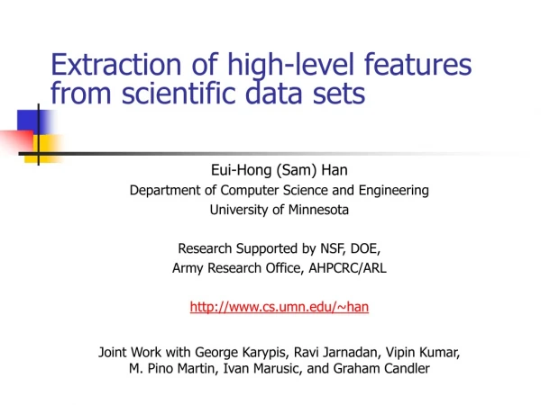
Extraction of high-level features from scientific data sets

1. Extraction of high-level features from scientific data sets Eui-Hong (Sam) Han Department of Computer Science and Engineering University of Minnesota Research Supported by NSF, DOE, Army Research Office, AHPCRC/ARL http://www.cs.umn.edu/~han Joint Work with George Karypis, Ravi Jarnadan, Vipin Kumar, M. Pino Martin, Ivan Marusic, and Graham Candler

2. Scientific Data Sets • Large amount of raw data available from scientific domains • direct numerical simulations • NASA satellite observations/climate data • genomics • astronomy • How do we apply existing data mining techniques on these data sets?

3. Direct Numerical Simulation

4. El Nino Effects on the Biosphere C Potter and S. Klooster, NASA Ames Research Center

5. categorical categorical continuous class C4.5 Decision Trees Splitting Attribute Refund Yes No NO MarSt Married Single, Divorced TaxInc NO < 80K > 80K YES NO The splitting attribute is determined based on the Gini index or Entropy gain

6. Associations in Transaction Data Sets Dependency relations among collection of items appearing in transactions. • Frequent Item Sets: set of items that appear frequently together in transactions • |{Diaper, Milk}| = 3 • |{Diaper,Milk,Beer}| = 2 • Association Rules • Application Areas • Inventory/Shelf planning • Marketing and Promotion

7. Challenges of Applying Data Mining Techniques • How do we construct transactions? • in the presence of spatial attributes • in the presence of temporal attributes • What are “interesting’’ events in the transactions? • high level objects (e.g., vortex in simulation) • high level features (e.g., El Nino event in weather data) • How do we find knowledge from the transactions and interesting events?

8. Feature extraction from simulation data using decision trees 3-D isosurface of “swirl strength” Velocity normal to the wall on XY plane (at z=30) Which features are important for high upward velocity on the XY plane?

9. Grid point z y x Transaction construction • Given 3D swirl strength data and corresponding velocity data on the XY plane at each simulation time step. • swirl_strength(x,y,z) = 1 iff swirl strength at (x,y,z) > swirl threshold • velocity(x,y) = 1 iff upward velocity at (x,y) > velocity threshold velocity(x,y) = -1 iff downward velocity at (x,y) > velocity threshold • A transaction corresponds to a grid point on the XY plane at one time step. • Class is velocity of the grid point • Attributes correspond to swirl_strength(x,y,z) of the neighbors of the point ss(-1:1,2:3,4:7)

10. C4.5 results on the simulation data • Given simulation data of 1000 time points • first 500 time points were used for training set • second 500 time points were used for testing set • 10% sample of class 0 transactions • 95% classification accuracy • Recall/precision of 0.83/0.95 for class -1 and 0.67/0.93 for class 1

11. Discovered Rules & Features F1 => class 1 • (F1:ss(0,1,0) = 0 & ss(-1,-2:-3,-4:-7) = 1 & ss(-1:1,-2:-3,8:15) = 1 & ss(1,0,2:3) = 1) => class 1 • (F2: ss(0,1,0) = 0 & ss(-1:1,-2:-3,-4:-7) = 0 & ss(1,-1,-2:-3) = 0 & ss(2:3,2:3,-16:-31) = 0 & ss(1:0:-1) = 0) => class 0 • (F3: ss(0,1,0) = 0 & …. & ss(-2:-3,2:3,8:15) = 1) => class -1

12. How to use the discovered features? • Finding association rules • (F1, Vortex Type A) => (high energy, F5) • Finding sequential patterns • (F2, Vortex Type A) => (F3, Vortex Type B) => (class 1) • Finding clusters of upward velocity points based on discovered features, vortex types, and other variables.

13. Finding functional relationships • Regression techniques find global and/or contiguous relationships • Association rules find • local relationships with • sufficient support http://www.cgd.ucar.edu/stats/web.book/index.html • Need to find global • relationships that have • sufficient support

14. (1,-1) y=x+1 d d Transformed space Solution in the original space c Original space c b b a a Finding functional relationships using duality transformation • Duality transformation in 2D space • Point p=(a,b) => line p’ : y=ax-b • Line l: y=Ax-B => point l’=(A,B) • p on l => l’ on p’ • l=line between p and q => l’ = intersection of p’ and q’

15. Finding functional relationships using duality transformation • Given n points in d dimension, find all hyperplanes that have at least k number of data points on the hyperplane. • In the transformed space, given n hyperplanes in d dimension, find all the intersection points that have at least k hyperplanes. • Efficient algorithms to find intersections exist. • These intersections corresponds to the hyperplanes in the original space.

16. Functional relationships in synthetic data sets • 1054 data points and 2000 noise points • Found all the intersections of two points in the transformed space • Drew a slope-sensitive grid on the transformed space • Selected grids that have above threshold intersection points • Plotted the average corresponding line of each selected grid on the original point space

17. Functional relationships in Ozone study • Case Studies in Environmental Statistics, by D. Nychka, W. Piegorsch, and L. Cox (http://www.cgd.ucar.edu/stats/web.book/index.html) • daily maximum ozone measurement as parts per million (ppm), temperature, wind speed, etc from 04/01/81 to 10/31/91 over Chicago area • found the most dominant functional relationship wspd = 0.09*ozone - 0.14*temp + 2.9

18. Functional relationships in Ozone study • Found a less dominant functional relationship wspd = 0.5*ozone - 0.4*temp + 3.03 • This functional relationship covers only subset of data points on the lower levels of ozone measurement • Potential follow up studies • what is unique about this functional relationship? • is there any unique characteristics of the supporting set?

19. How to use discovered functional relationships? • Discover decision rules using both functional relationships and original variables. • (supporting R1) and (Humidity > 80%) => class high-ozone-level • Discover association rules and sequential patterns with these functional relationships • ((supporting R2), Vortex Type A) => (high upward velocity) • Comparative analysis of supporting sets of R1 and R2.

20. Research Issues in Finding Functional Relationships • Non-linear relationships can be found by introducing extra variables like x^2, sin(x), exp(x) for every variable x. • Spatial relationships can be found by introducing variables of neighbors. • Temporal relationships can also be found by associating time stamp with variables.

21. Research Issues in Finding Functional Relationships • High computational cost of O(n^d) where n is the number of data points and d is the number of variables in the relationships. • Approximation algorithms are needed. • Clustering data points to reduce n • Focusing methods where inexact solutions are found using faster algorithms and more accurate relationships are found focusing on these inexact solutions. • Iterative methods where the most dominant relationship is found first and less dominant relationships are found in the later iterations