Download
1 / 65
650 likes | 983 Views
Quantified formulas. Decision procedures – An algorithmic point of view Daniel Kroening and Ofer Strichman. Why do we need quantifiers ?. As always: more modeling power Examples of quantifiers usage: “ Everyone in the room has a friend”

E N D
Quantified formulas Decision procedures – An algorithmic point of view Daniel Kroening and Ofer Strichman Decision Procedures - An algorithmic point of view
Why do we need quantifiers ? • As always: more modeling power • Examples of quantifiers usage: • “Everyone in the room has a friend” • “There is a person in the room that all of his cars are red” • “There is not more than one person in the room that earns more than $1M” Decision Procedures - An algorithmic point of view
Quantifiers in Math… • For any integer x there is a smaller integer y 8x2Z9y2Z. y < x X • Reverse claim: There exists an integer y such that any integer x is greater than y 9y2Z8x2Z. y < x£ • (Bertrand’s postulate) For any natural number greater than 1 there is a prime number p such that n < p < 2n 8n2N. 9p2N. n >1 ! (isprime(p) Æn < p < 2n) Decision Procedures - An algorithmic point of view
Actually… • Satisfiability of (x1,,xn) = does there exist an interpretation of x1,,xn that satisfies ? • Validity of (x1,,xn) = does it hold that all interpretation of x1,,xn satisfy ? • Conclusion: what we did so far (satisfiability, validity) is non-alternating quantification. Decision Procedures - An algorithmic point of view
Example: Quantified Propositional Logic • Better known as Quantified Boolean Formulas (QBF) formula: var | :formula | formulaÇformula | ( formula ) | T | F|8 var. (formula) | 9 var. (formula) 8x. (xÇ9y. (y!x)) 8x. (9y. ((xÇ:y) Æ (:xÇy)) Æ9y. ((:yÇ:x) Æ (xÇy))) X X Binding scope of y Decision Procedures - An algorithmic point of view
Prenex Normal-Form (PNF) • Formulas in PNF look like this: ’: Q[n]V[n]. .Q[1]V[1].Quantifier-free formula where Q[i] 2 {8,9} and V[i] is a variable. • Every quantified formula can be transformed to PNF while preserving validity. How ? prefix Decision Procedures - An algorithmic point of view
Prenex Normal Form (PNF) • Eliminate ! and $ (transform to ÇÆ:) • Push negations inside using::8x. $9x. ::9x. $8x. : • If there are name conflicts across scopes, solve with renaming. • Move quantifiers out by using recursively rules such as: • Q1x. 1(x) Æ Q2y. 2(y) $ Q1x. Q2y. (1(x) Æ2(y)) Qi2{8,9} • Q1x. 1(x) Ç Q2y. 2(y) $ Q1 x. Q2y. (1(x) Ç2(y)) Qi2{8,9} • 1Æ9x. 2(x) $9 x. (1Æ2(x)) where x does not appear in 1 • 1Æ8x. 2(x) $8x. (1Æ2(x)) where x does not appear in 1 • 8x. 1(x) Æ8x. 2(x) $8x. (1(x) Æ2(x)) • 9x. 1(x) Ç9x. 2(x) $9x. (1(x) Ç2(x)) Decision Procedures - An algorithmic point of view
Prenex Normal Form (PNF): example :9x. : (9y. ((y!x) Æ (: x Çy)) Æ:8y. ((yÆx) Ç (:xÆ: y))) 1,2. Eliminate !, push negations inside: 8x. (9y. ((:yÇx) Æ (: x Çy)) Æ9y. ((:yÇ:x) Æ (xÇy))) 3. Renaming: 8x. (9y1. ((:y1 Çx) Æ (: x Çy1)) Æ9y2. ((:y2Ç:x) Æ (xÇy2))) 4. Move quantifiers to front: 8x. 9y1. 9y2. (xÇ:y1) Æ (:xÇy1) Æ (:y2Ç:x) Æ (xÇy2) Decision Procedures - An algorithmic point of view
Why eliminating 9x. ÆiLi is enough • A procedure for eliminating an existential quantifier applied to a conjunction of literals is enough, because: • Given a formula , write it in DNF. • Use the fact that • Eliminate universal quantifiers using the fact8x. $:9x. : Decision Procedures - An algorithmic point of view
Quantifier Elimination • Examples first, generalization later. • Example #1: Quantified Boolean Formulas (QBF) • Example #2: Quantified Linear Arithmetic (QLA) Decision Procedures - An algorithmic point of view
Example #1: QBF • Examples of Quantified Boolean Formula : u e.(uÇ:e)(:uÇe) : e4e5 u1u2u3 e1e2e3. f(e1,e2,e3,e4,e5,u1,u2,u3) • QBF Problem: is valid? • P-Space Complete, theoretically harder than NP-Complete problems such as SAT. Decision Procedures - An algorithmic point of view
Motivations • QBF has practical applications: • AI Planning • Sequential circuit verification • … Decision Procedures - An algorithmic point of view
a Ç b Ç c’ Ç f g Ç h’ Ç c Ç f a Ç b Ç g Ç h’ a Ç b Ç g Ç h’Ç f Solving QBF with projection: 9 • Eliminate 9x. by projecting x on variables in higher quantification levels (their scope includes x’s scope). • In Propositional Logic projection can be done with Resolution. • Resolution example: Decision Procedures - An algorithmic point of view
Solving QBF with projection: 8 • Transform 8 to 9 via: (8x. )$ (:9x. :) • CNF is easier than general formulas: 8u1u2 9e18u3(u1Ç:e1)(:u1Çe1)(u2Ç:u3Ç:e1) 8u1u2 9e1:9u3 :((u1Ç:e1)(:u1Çe1)(u2Ç:u3Ç:e1)) 8u1u2 9e1:9u3 ((:u1Æe1)Ç(u1Æ:e1)Ç (:u2Æu3Æe1)) 8u1u2 9e1:((:u1Æe1)Ç(u1Æ:e1)Ç (:u2Æ(9u3. u3)Æe1)) 8u1u2 9e1 :((:u1Æe1)Ç(u1Æ:e1)Ç (:u2Æe1)) 8u1u2 9e1 (u1Ç:e1)(:u1Çe1)(u2Ç:e1) Suffix is DNF Replace with true Back to CNF Decision Procedures - An algorithmic point of view Shortcut for CNF formulas: simply erase universally quantified variables!
Resolution Based QBF Algorithm 8u1u29e18u39e3e2(u1Ç:e1)(:u1Ç:e2Çe3)(u2Ç:u3Ç:e1)(e1Çe2)(e1Ç:e3) 8u1u29e18u39e3 (u1Ç:e1)(:u1Çe3Çe1)(u2Ç:u3Ç:e1)(e1Ç:e3) 8u1u29e18u3 (u1Ç:e1)(:u1Çe1)(u2Ç:u3Ç:e1) 8u1u29e1(u1Ç:e1)(:u1Çe1)(u2Ç:e1) 8u1u2(:u1Çu2) FALSE Decision Procedures - An algorithmic point of view
Example #2: Quantified Linear Arithmetic formula = predicate | formulaÇformula | :formula | (formula) | 8 var. formula | 9 var. formula predicate = i ai xi·c 8x.9y.9z. (y+1 ·xÆz+1 ·yÆ 2x+1 ·z) Decision Procedures - An algorithmic point of view
Solving QLA with projection • Eliminate 9x. by projecting x. • In Linear Arithmetic over R projection can be done with Fourier-Motzkin elimination. • Fourier-Motzkin method to eliminate a variablexn:- for each pair of constraints: i=1..n-1ai’xi < xn < i=1..n-1aixi add a constrainti=1..n-1ai’xi < i=1..n-1aixi - in the end remove all constraints involving xn. Decision Procedures - An algorithmic point of view
Fourier Motzkin: example. Eliminate y: Solving QLA with projection 2y· 2z+ 4 y· 3z+ 3 Æ x+ 1 ·yÆ x+ 1 ·z+ 2 Æ x+ 1 · 3z+ 3 Decision Procedures - An algorithmic point of view
Quantifier elimination - example 8x.9y.9z. (y+1 ·xÆz+1 ·yÆ 2x+1 ·z) 8x.9y. (y+1 ·xÆ 2x+1 ·y-1 ) 8x. (2x+2 ·x-1) // transform to 9 :9x.: (2x+2 ·x-1) :9x.x > -3 :true false Decision Procedures - An algorithmic point of view
Quantifier elimination by projection: summary • Given a PNF formula f = Q[n]V[n]Q[1]V[1] For i = 1 .. n { if Q[i] =9then = project(,V[i]) else =:project(:,V[i]) } Return Decision Procedures - An algorithmic point of view
More about QBF • Example of using QBF (the diameter problem) • A search-based procedure for QBF. Acknowledgement: QBF slides borrowed from S. Malik Decision Procedures - An algorithmic point of view
initial state: S0 S1 S1 S2 S2 step 1: S1, S2 step 2: S3, S4 S0 S0 S3 S3 step 3: S5 S5 S5 S4 S4 The State Space Diameter Problem diameter = 3 Start from the initial states, the minimum number of steps needed to visit every reachable state Decision Procedures - An algorithmic point of view
Why is the Diameter Problem important? • Bounded model checking (BMC): search for a ‘bad’ state up to k steps from an initial step. • BMC can be formulated as SAT. Increasing k makes is harder. • Q: how deep should we go ? • A: as deep as the diameter • The diameter can be found by solving a QBF problem Decision Procedures - An algorithmic point of view
I1 In In+1 Combinational Logic Combinational Logic Combinational Logic O1 On On+1 I1’ In’ Combinational Logic Combinational Logic O1’ On’ Circuit Constructed for the Diameter Problem The idea: prove that for every state reachable in k+1 steps, there exists inputs that drive the model to this state earlier. Decision Procedures - An algorithmic point of view
I1 In In+1 Combinational Logic Combinational Logic Combinational Logic O1 On On+1 I1’ In’ Combinational Logic Combinational Logic O1’ On’ Some Terminology for the Formulations Variables: V Circuit consistency condition: C(V) Decision Procedures - An algorithmic point of view
I1 In In+1 Combinational Logic Combinational Logic Combinational Logic O1 On On+1 I1’ In’ Combinational Logic Combinational Logic O1’ On’ Some Terminology for the Formulations Variables: V’ Circuit consistency condition: C(V’) Decision Procedures - An algorithmic point of view
I1 In In+1 Combinational Logic Combinational Logic Combinational Logic O1 On On+1 I1’ In’ Combinational Logic Combinational Logic O1’ On’ QBF Formulation C(V) C(V’) OtherV variables V’ variables, incl. inputs Vinputs Decision Procedures - An algorithmic point of view
Another way to project Boolean variables • Shannon expansion:9x. = |x=0 Ç|x=1 8x. = |x=0 Æ|x=1 // can be derived from 8x. = :9x.: • The same applies for all finite-range variables. • Applying 9x., where in CNF $ resolution • But: does not need to be in CNF, and there is no need to transform the formula to DNF. Decision Procedures - An algorithmic point of view
Projection for non-CNF formulas: example 9y8z9x. (yÇ (xÆz)) 9y8z. (yÇ (xÆz))|x=0 Ç (yÇ (xÆz))|x=1 9y8z. ((y)Ç (yÇz)) 9y:9z. (:yÆ:z) 9y. : ((:yÆ:z)|z=0 Ç (:yÆ:z)|z=1) 9y. : (:y) True Decision Procedures - An algorithmic point of view
Search Based QBF Algorithms • Work by gradually assigning variables • A partial assignment [KGS98] M. Cadoli, A. Giovanardi, M. Schaerf. An Algorithm to Evaluate Quantified Boolean Formulae. In Proc. of 16th National Conference on Artificial Intelligence (AAAI-98) Decision Procedures - An algorithmic point of view
Search Based QBF Algorithms • Work by gradually assigning variables • A partial assignment • Undetermined • Continue search [KGS98] M. Cadoli, A. Giovanardi, M. Schaerf. An Algorithm to Evaluate Quantified Boolean Formulae. In Proc. of 16th National Conference on Artificial Intelligence (AAAI-98) Decision Procedures - An algorithmic point of view
Search Based QBF Algorithms • Work by gradually assigning variables • A partial assignment • Undetermined • Conflict • Backtrack • Record the reason [KGS98] M. Cadoli, A. Giovanardi, M. Schaerf. An Algorithm to Evaluate Quantified Boolean Formulae. In Proc. of 16th National Conference on Artificial Intelligence (AAAI-98) Decision Procedures - An algorithmic point of view
Search Based QBF Algorithms • Work by gradually assigning variables • A partial assignment • Undetermined • Conflict • Satisfied • Backtrack • Determine the covered satisfying space [KGS98] M. Cadoli, A. Giovanardi, M. Schaerf. An Algorithm to Evaluate Quantified Boolean Formulae. In Proc. of 16th National Conference on Artificial Intelligence (AAAI-98) Decision Procedures - An algorithmic point of view
Search Based QBF Algorithms • Work by gradually assigning variables • A partial assignment • Undetermined • Conflict • Satisfied • The majority of QBF solvers are search based, the DPLL algorithm is an example of this Decision Procedures - An algorithmic point of view
Basic DPLL Flow for QBF eu (eÇu)(:eÇ:u) Unknown True (1) False(0) Decision Procedures - An algorithmic point of view
Basic DPLL Flow for QBF eu (eÇu)(:eÇ:u) e = 0 Unknown True (1) False(0) Decision Procedures - An algorithmic point of view
Basic DPLL Flow for QBF Existential quantification eu (eÇu)(:eÇ:u) Universal quantification e = 0 Satisfying Node Unknown True (1) u = 1 False(0) Decision Procedures - An algorithmic point of view
Basic DPLL Flow for QBF eu (eÇu)(:eÇ:u) e = 0 Backtrack Unknown True (1) u = 1 False(0) Decision Procedures - An algorithmic point of view
Basic DPLL Flow for QBF eu (eÇu)(:eÇ:u) e = 0 Unknown True (1) u = 1 u = 0 False(0) Decision Procedures - An algorithmic point of view
Basic DPLL Flow for QBF eu (eÇu)(:eÇ:u) e = 0 Unknown True (1) u = 1 u = 0 False(0) Decision Procedures - An algorithmic point of view
Basic DPLL Flow for QBF eu (eÇu)(:eÇ:u) e = 1 e = 0 Unknown True (1) u = 1 u = 0 False(0) Decision Procedures - An algorithmic point of view
Basic DPLL Flow for QBF eu (eÇu)(:eÇ:u) e = 1 e = 0 Unknown True (1) u = 1 u = 1 u = 0 False(0) Decision Procedures - An algorithmic point of view
Basic DPLL Flow for QBF eu (eÇu)(:eÇ:u) e = 1 e = 0 Conflicting Node Unknown True (1) u = 1 u = 1 u = 0 False(0) Decision Procedures - An algorithmic point of view
Basic DPLL Flow for QBF eu (eÇu)(:eÇ:u) e = 1 e = 0 Unknown True (1) u = 1 u = 1 u = 0 False(0) Decision Procedures - An algorithmic point of view
Basic DPLL Flow for QBF False eu (eÇu)(:eÇ:u) e = 1 e = 0 Unknown True (1) u = 1 u = 1 u = 0 False(0) Decision Procedures - An algorithmic point of view
Basic DPLL Flow for QBF ue (uÇe)(:uÇ:e) Unknown True (1) False(0) Decision Procedures - An algorithmic point of view
Basic DPLL Flow for QBF ue (uÇe)(:uÇ:e) u = 1 Unknown True (1) False(0) Decision Procedures - An algorithmic point of view
Basic DPLL Flow for QBF ue (uÇe)(:uÇ:e) u = 1 Unknown True (1) e = 1 False(0) Decision Procedures - An algorithmic point of view
Basic DPLL Flow for QBF ue (uÇe)(:uÇ:e) u = 1 Unknown True (1) e = 1 e = 0 False(0) Decision Procedures - An algorithmic point of view
Basic DPLL Flow for QBF ue (uÇe)(:uÇ:e) u = 1 Unknown True (1) e = 1 e = 0 False(0) Decision Procedures - An algorithmic point of view