How will execution time grow with SIZE?

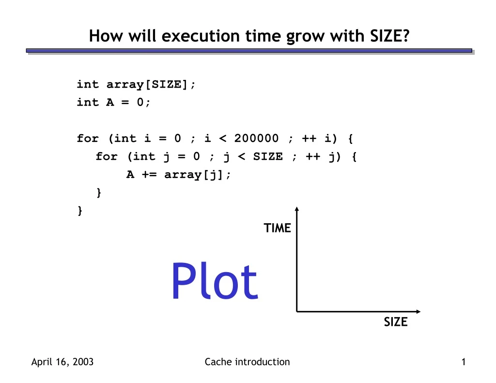
1. How will execution time grow with SIZE? int array[SIZE]; int A = 0; for (int i = 0 ; i < 200000 ; ++ i) { for (int j = 0 ; j < SIZE ; ++ j) { A += array[j]; } } TIME Plot SIZE Cache introduction

2. Actual Data from remsun2.ews.uiuc.edu Cache introduction

3. Memory Processor Input/Output Welcome to Part 3: Memory Systems and I/O • We’ve already seen how to make a fast processor. How can we supply the CPU with enough data to keep it busy? • The rest of course focuses on memory and input/output issues, which are frequently bottlenecks that limit the performance of a system. • We’ll start off by looking at memory systems for the next two weeks, and then turn to I/O for a week. • How caches can dramatically improve the speed of memory accesses. • How virtual memory provides security and ease of programming • How processors, memory and peripheral devices can be connected

4. Today: Cache introduction • Today we’ll answer the following questions. • What are the challenges of building big, fast memory systems? • What is a cache? • Why caches work? (answer: locality) • How are caches organized? • Where do we put things -and- how do we find them?

5. Today: Cache introduction

6. Large and fast • Today’s computers depend upon large and fast storage systems. • Large storage capacities are needed for many database applications, scientific computations with large data sets, video and music, and so forth. • Speed is important to keep up with our pipelined CPUs, which may access both an instruction and data in the same clock cycle. Things get become even worse if we move to a superscalar CPU design. • So far we’ve assumed our memories can keep up and our CPU can access memory twice in one cycle, but as we’ll see that’s a simplification. Cache introduction

7. Small or slow • Unfortunately there is a tradeoff between speed, cost and capacity. • Fast memory is too expensive for most people to buy a lot of. • But dynamic memory has a much longer delay than other functional units in a datapath. If every lw or sw accessed dynamic memory, we’d have to either increase the cycle time or stall frequently. • Here are rough estimates of some current storage parameters. Cache introduction

8. CPU A little static RAM (cache) Lots of dynamic RAM Introducing caches • Wouldn’t it be nice if we could find a balance between fast and cheap memory? • We do this by introducing a cache, which is a small amount of fast, expensive memory. • The cache goes between the processor and the slower, dynamic main memory. • It keeps a copy of the most frequently used data from the main memory. • Memory access speed increases overall, because we’ve made the common case faster. • Reads and writes to the most frequently used addresses will be serviced by the cache. • We only need to access the slower main memory for less frequently used data. Cache introduction

9. The principle of locality • It’s usually difficult or impossible to figure out what data will be “most frequently accessed” before a program actually runs, which makes it hard to know what to store into the small, precious cache memory. • But in practice, most programs exhibit locality, which the cache can take advantage of. • The principle of temporal locality says that if a program accesses one memory address, there is a good chance that it will access the same address again. • The principle of spatial locality says that if a program accesses one memory address, there is a good chance that it will also access other nearby addresses. Cache introduction

10. Temporal locality in programs • The principle of temporal locality says that if a program accesses one memory address, there is a good chance that it will access the same address again. • Loops are excellent examples of temporal locality in programs. • The loop body will be executed many times. • The computer will need to access those same few locations of the instruction memory repeatedly. • For example: • Each instruction will be fetched over and over again, once on every loop iteration. Loop: lw $t0, 0($s1) add $t0, $t0, $s2 sw $t0, 0($s1) addi $s1, $s1, -4 bne $s1, $0, Loop Cache introduction

11. Temporal locality in data • Programs often access the same variables over and over, especially within loops. Below, sum and i are repeatedly read and written. • Commonly-accessed variables can sometimes be kept in registers, but this is not always possible. • There are a limited number of registers. • There are situations where the data must be kept in memory, as is the case with shared or dynamically-allocated memory. sum = 0; for (i = 0; i < MAX; i++) sum = sum + f(i); Cache introduction

12. Spatial locality in programs • The principle of spatial locality says that if a program accesses one memory address, there is a good chance that it will also access other nearby addresses. • Nearly every program exhibits spatial locality, because instructions are usually executed in sequence—if we execute an instruction at memory location i, then we will probably also execute the next instruction, at memory location i+1. • Code fragments such as loops exhibit both temporal and spatial locality. sub $sp, $sp, 16 sw $ra, 0($sp) sw $s0, 4($sp) sw $a0, 8($sp) sw $a1, 12($sp) Cache introduction

13. Spatial locality in data • Programs often access data that is stored contiguously. • Arrays, like a in the code on the top, are stored in memory contiguously. • The individual fields of a record or object like employee are also kept contiguously in memory. • Can data have both spatial and temporal locality? sum = 0; for (i = 0; i < MAX; i++) sum = sum + a[i]; employee.name = “Homer Simpson”; employee.boss = “Mr. Burns”; employee.age = 45; Cache introduction

14. CPU A little static RAM (cache) Lots of dynamic RAM How caches take advantage of temporal locality • The first time the processor reads from an address in main memory, a copy of that data is also stored in the cache. • The next time that same address is read, we can use the copy of the data in the cache instead of accessing the slower dynamic memory. • So the first read is a little slower than before since it goes through both main memory and the cache, but subsequent reads are much faster. • This takes advantage of temporal locality—commonly accessed data is stored in the faster cache memory. Cache introduction

15. CPU A little static RAM (cache) Lots of dynamic RAM How caches take advantage of spatial locality • When the CPU reads location i from main memory, a copy of that data is placed in the cache. • But instead of just copying the contents of location i, we can copy several values into the cache at once, such as the four bytes from locations i through i + 3. • If the CPU later does need to read from locations i + 1, i + 2 or i + 3, it can access that data from the cache and not the slower main memory. • For example, instead of reading just one array element at a time, the cache might actually be loading four array elements at once. • Again, the initial load incurs a performance penalty, but we’re gambling on spatial locality and the chance that the CPU will need the extra data. Cache introduction

16. Other kinds of caches • The idea of caching is not specific to architecture. • caches are used in many other situations. Web browser File system Google pre-computed queries Harddrive TLB Fridge Cache introduction

17. Other kinds of caches • The general idea behind caches is used in many other situations. • Networks are probably the best example. • Networks have relatively high “latency” and low “bandwidth,” so repeated data transfers are undesirable. • Browsers like Netscape and Internet Explorer store your most recently accessed web pages on your hard disk. • Administrators can set up a network-wide cache, and companies like Akamai also provide caching services. • A few other examples: • Many processors have a “translation lookaside buffer,” which is a cache dedicated to virtual memory support. • Operating systems may store frequently-accessed disk blocks, like directories, in main memory... and that data may then in turn be stored in the CPU cache! Cache introduction

18. Definitions: Hits and misses • A cache hit occurs if the cache contains the data that we’re looking for. Hits are good, because the cache can return the data much faster than main memory. • A cache miss occurs if the cache does not contain the requested data. This is bad, since the CPU must then wait for the slower main memory. • There are two basic measurements of cache performance. • The hit rate is the percentage of memory accesses that are handled by the cache. • The miss rate (1 - hit rate) is the percentage of accesses that must be handled by the slower main RAM. • Typical caches have a hit rate of 95% or higher, so in fact most memory accesses will be handled by the cache and will be dramatically faster. • In future lectures, we’ll talk more about cache performance. • Today we’ll talk about implementation! Cache introduction

19. Block index 8-bit data 000 001 010 011 100 101 110 111 A simple cache design • Caches are divided into blocks, which may be of various sizes. • The number of blocks in a cache is usually a power of 2. • For now we’ll say that each block contains one byte. This won’t take advantage of spatial locality, but we’ll do that next time. • Here is an example cache with eight blocks, each holding one byte. Cache introduction

20. Four important questions 1. When we copy a block of data from main memory to the cache, where exactly should we put it? 2. How can we tell if a word is already in the cache, or if it has to be fetched from main memory first? 3. Eventually, the small cache memory might fill up. To load a new block from main RAM, we’d have to replace one of the existing blocks in the cache... which one? 4. How can write operations be handled by the memory system? • Questions 1 and 2 are related—we have to know where the data is placed if we ever hope to find it again later! Cache introduction

21. Where should we put data in the cache? • A direct-mapped cache is the simplest approach: each main memory address maps to exactly one cache block. • For example, on the right is a 16-byte main memory and a 4-byte cache (four 1-byte blocks). • Memory locations 0, 4, 8 and 12 all map to cache block 0. • Addresses 1, 5, 9 and 13 map to cache block 1, etc. • How can we compute this mapping? Memory Address 0 1 2 3 4 5 6 7 8 9 10 11 12 13 14 15 Index 0 1 2 3 Cache introduction

22. Memory Address 0 1 2 3 4 5 6 7 8 9 10 11 12 13 14 15 Index 0 1 2 3 It’s all divisions… • One way to figure out which cache block a particular memory address should go to is to use the mod (remainder) operator. • If the cache contains 2k blocks, then the data at memory address i would go to cache block index i mod 2k • For instance, with the four-block cache here, address 14wouldmap to cache block 2. 14 mod 4 = 2 Cache introduction

23. …or least-significant bits • An equivalent way to find the placement of a memory address in the cache is to look at the least significant k bits of the address. • With our four-byte cache we would inspect the two least significant bits of our memory addresses. • Again, you can see that address 14 (1110 in binary) maps to cache block 2 (10 in binary). • Taking the least k bits of a binary value is the same as computing that value mod 2k. Memory Address 0000 0001 0010 0011 0100 0101 0110 0111 1000 1001 1010 1011 1100 1101 1110 1111 Index 00 01 10 11 Cache introduction

24. Memory Address 0 1 2 3 4 5 6 7 8 9 10 11 12 13 14 15 Index 0 1 2 3 How can we find data in the cache? • The second question was how to determine whether or not the data we’re interested in is already stored in the cache. • If we want to read memory address i, we can use the mod trick to determine which cache block would contain i. • But other addresses might also map to the same cache block. How can we distinguish between them? • For instance, cache block 2 could contain data from addresses 2, 6, 10or14. Cache introduction

25. 0000 0001 0010 0011 0100 0101 0110 0111 1000 1001 1010 1011 1100 1101 1110 1111 Index Tag Data 00 01 10 11 00 ?? 01 01 Adding tags • We need to add tags to the cache, which supply the rest of the address bits to let us distinguish between different memory locations that map to the same cache block. Cache introduction

26. 0000 0001 0010 0011 0100 0101 0110 0111 1000 1001 1010 1011 1100 1101 1110 1111 Index Tag Data 00 01 10 11 00 11 01 01 Adding tags • We need to add tags to the cache, which supply the rest of the address bits to let us distinguish between different memory locations that map to the same cache block. Cache introduction

27. Main memory address in cache block Index Tag Data 00 + 00 = 0000 11 + 01 = 1101 01 + 10 = 0110 01 + 11 = 0111 00 01 10 11 00 11 01 01 Figuring out what’s in the cache • Now we can tell exactly which addresses of main memory are stored in the cache, by concatenating the cache block tags with the block indices. Cache introduction

28. Valid Bit Main memory address in cache block Index Tag Data 00 + 00 = 0000 Invalid ??? ??? 00 01 10 11 1 0 0 1 00 11 01 01 One more detail: the valid bit • When started, the cache is empty and does not contain valid data. • We should account for this by adding a valid bit for each cache block. • When the system is initialized, all the valid bits are set to 0. • When data is loaded into a particular cache block, the corresponding valid bit is set to 1. • So the cache contains more than just copies of the data in memory; it also has bits to help us find data within the cache and verify its validity. Cache introduction

29. Valid Bit Main memory address in cache block Index Tag Data 00 + 00 = 0000 Invalid Invalid 01 + 11 = 0111 00 01 10 11 1 0 0 1 00 11 01 01 One more detail: the valid bit • When started, the cache is empty and does not contain valid data. • We should account for this by adding a valid bit for each cache block. • When the system is initialized, all the valid bits are set to 0. • When data is loaded into a particular cache block, the corresponding valid bit is set to 1. • So the cache contains more than just copies of the data in memory; it also has bits to help us find data within the cache and verify its validity. Cache introduction

30. Index Valid Tag Data Address (32 bits) 0 1 2 3 ... ... 1022 1023 22 10 Index To CPU Tag Hit = What happens on a cache hit • When the CPU tries to read from memory, the address will be sent to a cache controller. • The lowest k bits of the address will index a block in the cache. • If the block is valid and the tag matches the upper (m-k) bits of the m-bit address, then that data will be sent to the CPU. • Here is a diagram of a 32-bit memory address and a 210-byte cache. Cache introduction

31. What happens on a cache miss • The delays that we’ve been assuming for memories (e.g., 2ns) are really assuming cache hits. • If our CPU implementations accessed main memory directly, their cycle times would have to be much larger. • Instead we assume that most memory accesses will be cache hits, which allows us to use a shorter cycle time. • However, a much slower main memory access is needed on a cache miss. The simplest thing to do is to stall the pipeline until the data from main memory can be fetched (and also copied into the cache). Cache introduction

32. Index Valid Tag Data Address (32 bits) 0 1 2 3 ... ... ... 22 10 Index Tag Data 1 Loading a block into the cache • After data is read from main memory, putting a copy of that data into the cache is straightforward. • The lowest k bits of the address specify a cache block. • The upper (m-k) address bits are stored in the block’s tag field. • The data from main memory is stored in the block’s data field. • The valid bit is set to 1. Cache introduction

33. What if the cache fills up? • Our third question was what to do if we run out of space in our cache, or if we need to reuse a block for a different memory address. • We answered this question implicitly on the last page! • A miss causes a new block to be loaded into the cache, automatically overwriting any previously stored data. • This is a least recently used replacement policy, which assumes that older data is less likely to be requested than newer data. • We’ll see a few other policies next week. Cache introduction

34. Summary • Today we studied the basic ideas of caches. • By taking advantage of spatial and temporal locality, we can use a small amount of fast but expensive memory to dramatically speed up the average memory access time. • A cache is divided into many blocks, each of which contains a valid bit, a tag for matching memory addresses to cache contents, and the data itself. • Next week we’ll look at some more advanced cache organizations and see how to measure the performance of memory systems. Cache introduction