Download
1 / 19
190 likes | 307 Views
Optimal Sample Designs for Mapping EMAP Data. Molly Leecaster, Ph.D. Idaho National Engineering & Environmental Laboratory Jennifer Hoeting, Ph. D. Colorado State University Kerry Ritter, Ph.D. Southern California Coastal Water Research Project. September 21, 2002. FUNDING SOURCE.

E N D
Optimal Sample Designs for Mapping EMAP Data Molly Leecaster, Ph.D. Idaho National Engineering & Environmental Laboratory Jennifer Hoeting, Ph. D. Colorado State University Kerry Ritter, Ph.D. Southern California Coastal Water Research Project September 21, 2002
FUNDING SOURCE • This presentation was developed under the STAR Research Assistance Agreement CR-829095 awarded by the U.S. Environmental Protection Agency (EPA) to Colorado State University. This presentation has not been formally reviewed by EPA. The views expressed here are solely those of its authors and the STARMAP Program. EPA does not endorse any products or commercial services mentioned in this presentation.
Outline of Presentation • EMAP data • Models for mapping • Optimal designs for each model • Future work
EMAP Data • Uses • Decision making • Hypothesis generation • Future sampling designs • Temporal models • Presentation • Posting Plots • CDF’s • Binary response: above/below threshold • Maps
Total DDT (ng/g) levels in Santa Monica Bay SCBPP ‘94 34.0 33.9 33.8 0.50 936.80 33.7 -118.8 -118.7 -118.6 -118.5 -118.4
Models to Map Binary EMAP Data • Kriging for geo-referenced data • Autologistic model for lattice data
Kriging • Indicator, probability, or disjunctive kriging for binary data • Geo-referenced data • May include covariates • Variogram to investigate spatial correlation structure • Kriging variance dependent on sample spacing and variance of response
Autologistic Model • Binary lattice data • May include covariates • Spatial correlation structure assumed: locally dependent Markov random field • Neighborhood defined as fixed pattern of surrounding grid cells • Precision of predictions depends on neighborhood structure, grid size, and variance of response • Bayesian estimation of model parameters and response
Optimal Sample Designs for Mapping EMAP Data • Optimal : Greatest precision for lowest sample cost • Optimal kriging sample spacing has been investigated, but not co-kriging • Optimal grid size for hexagon lattice is an open question • Triangular geo-referenced design is equivalent to hexagon lattice design
Optimal Spacing for Co-kriging • Kriging variance depends on • sample spacing • variograms • cross variograms
Optimal Grid for Lattice Model • Assume grid cells homogeneous • Too big: not homogeneous • Too small: wasted sampling resources • Assume spatial correlation depends on neighborhood, and thus grid cell size • Too big: spatial correlation only within grid cell • Too small: spatial correlation extends beyond neighborhood
Future Work • Data • Proposed approach
Data for Preliminary Work • Sediment total DDT from Santa Monica Bay, CA • 1994 Southern California Bight Pilot Project • EMAP design • 77 samples • Other surveys and routine monitoring data • Covariates • Depth • Co-kriging-predicted grain size (percent fines)
Proposed Approach • Autologistic model for hexagon lattice • program in S-Plus, R, or Win-Bugs • Develop measure of precision for autologistic model • akin to kriging variance • Determine optimal lattice for autologistic model • Determine optimal spacing for co-kriging • Compare precision, accuracy, and sample size between optimal autologistic and co-kriging designs • Generalize findings
Resources • Autologistic Program for S-Plus and C++ • http://www.stat.colostate.edu/~jah/software/ • Email addresses • leecmk@inel.gov • jah@stat.colostate.edu • kerryr@sccwrp.org