Download
1 / 32
330 likes | 451 Views
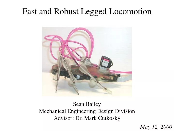
Fast and Robust Legged Locomotion. Sean Bailey Mechanical Engineering Design Division Advisor: Dr. Mark Cutkosky. May 12, 2000. Overview. Intro. Design. Biomimesis. Analysis. Conclusions. Introduction Functional Biomimesis Robot Design Model Analysis Conclusions.

E N D
Fast and Robust Legged Locomotion Sean Bailey Mechanical Engineering Design Division Advisor: Dr. Mark Cutkosky May 12, 2000
Overview Intro Design Biomimesis Analysis Conclusions • Introduction • Functional Biomimesis • Robot Design • Model Analysis • Conclusions
Fast, Robust Rough Terrain Traversal Intro Design Biomimesis Analysis Conclusions • Why? • Mine clearing • Urban Reconnaissance • Why legs? • Basic Design Goals • 1.5 body lengths per second • Hip-height obstacles • Simple
Traditional Approaches to Legged Systems Intro Design Biomimesis Analysis Conclusions • Statically stable • Tripod of support • Slow • Rough terrain • Dynamically stable • No support requirements • Fast • Smooth terrain
Biological Example Intro Design Biomimesis Analysis Conclusions • Death-head cockroach Blaberus discoidalis • Fast • Speeds of up to 10 body/s • Rough terrain • Can easily traverse fractal terrain of obstacles 3X hip height • Stability • Static and dynamic
Biomimesis Options Intro Design Biomimesis Analysis Conclusions Too complex! Functional Biomimesis “Biomimetic” configuration Extract fast rough terrain locomotion capabilities
Biological Inspiration Intro Design Biomimesis Analysis Conclusions • Control heirarchy • Passive component • Active component
Is Passive Enough? Intro Design Biomimesis Analysis Conclusions • Passive Dynamic Stabilization • No active stabilization • Geometry • Mechanical system properties
Geometry Intro Design Biomimesis Analysis Conclusions Cockroach Geometry Functional Biomimesis Robot Implementation • Passive Compliant Hip Joint • Effective Thrusting Force • Damped, Compliant Hip Flexure • Embedded Air Piston • Rotary Joint • Prismatic Joint
Sprawlita Intro Design Biomimesis Analysis Conclusions • Mass - .27 kg • Dimensions - 16x10x9 cm • Leg length - 4.5 cm • Max. Speed - 39cm/s 2.5 body/sec • Hip height obstacle traversal
Movie Intro Design Biomimesis Analysis Conclusions • Compliant hip • Alternating tripod • Stable running • Obstacle traversal
Mechanical System Properties Intro Design Biomimesis Analysis Conclusions • Prototype: Empirically tuned properties • Design for behavior ? Mechanical System Properties Modeling
“Simple” Model Full 3D model Symmetry assumption Planar model Intro Design Biomimesis Analysis Conclusions K, B, nom • Body has 3 planar degrees of freedom • x, z, theta • mass, inertia • 3 massless legs (per tripod) • rotating hip joint - damped torsional spring • prismatic leg joint - damped linear spring • 6 parameters per leg 18 parameters to tune - TOO MANY! k, b, nom
Simplest Locomotion Model g g Intro Design Biomimesis Analysis Conclusions • Body has 2 planar degrees of freedom • x, z • mass • 4 massless legs • freely rotating hip joint • prismatic leg joint - damped linear spring • 3 parameters per leg 6 parameters to tune, assuming symmetry k, b, nom Biped Biped Quadruped
Modeling assumptions g State x 0 Leg Set Leg Set Leg Set Leg Set 1 2 1 2 T T T T Time Stride Period = state trajectory Intro Design Biomimesis Analysis Conclusions • Time-Based Mode Transitions • Clock-driven motor pattern • “Groucho running”1 • One “reset” mode • Two sets of legs - Two modes • Symmetric - treat as one mode • Mode initial conditions • Nominal leg angles • Instant passive component compression 1 McMahon, et al 1987
Modeling assumptions g T T T T = state trajectory Intro Design Biomimesis Analysis Conclusions • Time-Based Mode Transitions • Clock-driven motor pattern • “Groucho running”1 • One “reset” mode • Two sets of legs - Two modes • Symmetric - treat as one mode • Mode initial conditions • Nominal leg angles • Instant passive component compression t = 2T- State x 0 Leg Set Leg Set Leg Set Leg Set 1 2 1 2 Time Stride Period 1 McMahon, et al 1987
Modeling assumptions g t = 2T+ State x 0 Leg Set Leg Set Leg Set Leg Set 1 2 1 2 T T T T Time Stride Period = state trajectory Intro Design Biomimesis Analysis Conclusions • Time-Based Mode Transitions • Clock-driven motor pattern • “Groucho running”1 • One “reset” mode • Two sets of legs - Two modes • Symmetric - treat as one mode • Mode initial conditions • Nominal leg angles • Instant passive component compression 1 McMahon, et al 1987
Modeling assumptions g t = 2T + 1/3T State x 0 Leg Set Leg Set Leg Set Leg Set 1 2 1 2 T T T T Time Stride Period = state trajectory Intro Design Biomimesis Analysis Conclusions • Time-Based Mode Transitions • Clock-driven motor pattern • “Groucho running”1 • One “reset” mode • Two sets of legs - Two modes • Symmetric - treat as one mode • Mode initial conditions • Nominal leg angles • Instant passive component compression 1 McMahon, et al 1987
Modeling assumptions g t = 2T + 2/3T State x 0 Leg Set Leg Set Leg Set Leg Set 1 2 1 2 T T T T Time Stride Period = state trajectory Intro Design Biomimesis Analysis Conclusions • Time-Based Mode Transitions • Clock-driven motor pattern • “Groucho running”1 • One “reset” mode • Two sets of legs - Two modes • Symmetric - treat as one mode • Mode initial conditions • Nominal leg angles • Instant passive component compression 1 McMahon, et al 1987
Modeling assumptions g t = 3T- State x 0 Leg Set Leg Set Leg Set Leg Set 1 2 1 2 T T T T Time Stride Period = state trajectory Intro Design Biomimesis Analysis Conclusions • Time-Based Mode Transitions • Clock-driven motor pattern • “Groucho running”1 • One “reset” mode • Two sets of legs - Two modes • Symmetric - treat as one mode • Mode initial conditions • Nominal leg angles • Instant passive component compression 1 McMahon, et al 1987
Modeling assumptions g t = 3T+ State x 0 Leg Set Leg Set Leg Set Leg Set 1 2 1 2 T T T T Time Stride Period = state trajectory Intro Design Biomimesis Analysis Conclusions • Time-Based Mode Transitions • Clock-driven motor pattern • “Groucho running”1 • One “reset” mode • Two sets of legs - Two modes • Symmetric - treat as one mode • Mode initial conditions • Nominal leg angles • Instant passive component compression 1 McMahon, et al 1987
Modeling assumptions g t = 3T + 1/3T State x 0 Leg Set Leg Set Leg Set Leg Set 1 2 1 2 T T T T Time Stride Period = state trajectory Intro Design Biomimesis Analysis Conclusions • Time-Based Mode Transitions • Clock-driven motor pattern • “Groucho running”1 • One “reset” mode • Two sets of legs - Two modes • Symmetric - treat as one mode • Mode initial conditions • Nominal leg angles • Instant passive component compression 1 McMahon, et al 1987
Non-linear analysis tools = state trajectory = fixed points xk+1 = xk = x* State x 0 Leg Set Leg Set Leg Set Leg Set 1 2 1 2 T T T T Time Stride Period = state trajectory Intro Design Biomimesis Analysis Conclusions • Discrete non-linear system • Fixed points • numerically integrate to find • exclude horizontal position information
Non-linear analysis tools = nominal trajectory Intro Design Biomimesis Analysis Conclusions • Floquet technique • Analyze perturbation response • Digital eigenvalues via linearization - examine stability • Use selective perturbations to construct M matrix Numerically Integrate
Non-linear analysis tools Intro Design Biomimesis Analysis Conclusions • Floquet technique
Perturbation Response Intro Design Biomimesis Analysis Conclusions
Analysis trends 0.075 2.8 Horizontal Velocity Recovery Rate 2.6 0.07 2.4 0.065 2.2 0.06 X_dot (m/s) 1/max[eig(M)] 2 0.055 1.8 0.05 1.6 0.045 1.4 0.04 1.2 6.5 7 7.5 8 8.5 9 9.5 10 Damping (N-s/m) Intro Design Biomimesis Analysis Conclusions • Relationships • damping vs. speed and “robustness” • stiffness, leg angles, leg lengths, stride period, etc • Use for design • select mechanical properties • select other parameters • Insight into the mechanism of locomotion
Design Example Robustness Speed Intro Design Biomimesis Analysis Conclusions Damping Damping Damping Stiffness Stiffness Stiffness Speed = 0 Speed = 13 cm/s Speed = 23.5 cm/s
Locomotion Insight Intro Design Biomimesis Analysis Conclusions • Body tends towardsequilibrium point • Parameters andmechanical propertiesdetermine how Trajectory Mode Equilibrium Statically Unstable Region Initial condition Leg Extension Limit Leg Pre- Compressions
Summary and Conclusions Intro Design Biomimesis Analysis Conclusions • Current leg systems are either fast or can handle rough terrain • Biology suggests emphasis on good mechanical design • enhances capability • simplifies control • Purely clock-driven systems can be fast and robust • Floquet technique can be used to indicate locomotion robustness • Trends can be established to improve design and provide insight
Future Work Intro Design Biomimesis Analysis Conclusions • Extend findings and insights to more complex models • Develop easily modeled 4th generation robot • Utilize sensor feedback in high level control • Examine other behaviors
Thanks! Intro Design Biomimesis Analysis Conclusions • Center for Design Research • Dexterous Manipulation Lab • Rapid Prototyping Lab • Mark Cutkosky • Jorge Cham, Jonathan Clark