Download
1 / 14
140 likes | 252 Views
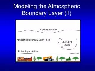
Extreme Values of Contaminant Concentration in the Atmospheric Boundary-Layer. Nils Mole ( University of Sheffield ) Thom Schopflocher Paul Sullivan ( University of Western Ontario ). Background. Typical diffusing plume.

E N D
Extreme Values of Contaminant Concentration in theAtmospheric Boundary-Layer Nils Mole (University of Sheffield) Thom Schopflocher Paul Sullivan (University of Western Ontario)
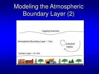
Background Typical diffusing plume The texture of the contaminant field consists of concentration in very thin sparsely distributed sheets.
Background… Fixed point measurements showing large peaks of concentration
High Concentration Tails pdf As the sum of two functions, Such that Moments of p(θ), For sufficiently large n,
Generalized Pareto Density function θ2 is the largest source concentration and a, k > 0. for sufficiently large n, Moment ratios are linear in 1/n, which should yield the values of a, k & θmax= a/k. ncan be found from
Experimental data Linear fits to the moment ratios for data from Sawford & Tivendale (1992). X is the downstream distance from the source, Z is the cross-stream distance from the centreline, and L is the mean plume width.
Experimental data The measured pdf of θ/Co (points), and GPD for fitted k and a values (curves). The right-hand panels show blow-ups of the tails. The dashed lines mark the estimated values of θc/Co.
Experimental data Variation with downwind distance X of the percentage range and area accounted for by the GPD, i.e. by θ ≥θc. (a) Range 1 − θc/θmax, (b) area A. The squares represent centreline measurements, and the crosses measurements at about 1L from the centreline.
Experimental data Variation on the centreline of GPD parameters (estimated from the data of Sawford & Tivendale 1992) with downstream distance X. (a) θmax/Co (squares), a/Co (triangles) and 10k (crosses), (b) θmax/Co (squares), and the approximation to θmax/Co in the no diffusion case based (curve).
Experimental data Variation across the plume of GPD parameters normalized by their centreline values. (a) θmax, (b) k, (c) a, (d) η. The line in (d) is that on which the normalized value of η equals C/Co.
Conclusions • Have shown the evolution of the high concentration tails, including θmax, in terms of lower order moments of pdf. • Further work (not shown here) using existing models of the moments provides a five parameter representation. • Some promising schemes for the solution of the moments equation, are currently under investigation.