Download
1 / 16
160 likes | 288 Views
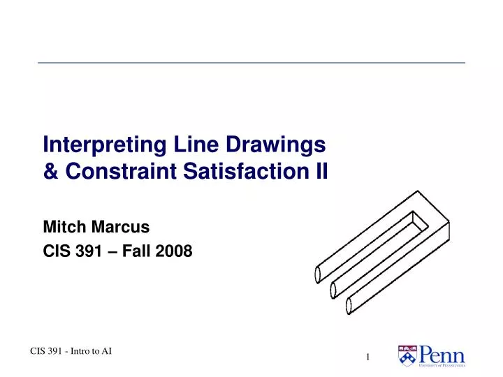
Interpreting Line Drawings & Constraint Satisfaction II. Mitch Marcus CIS 391 – Fall 2008. Constraint Propagation. Waltz’s insight: Pairs of adjacent junctions (junctions connected by a line) constrain each other’s interpretations!

E N D
Interpreting Line Drawings& Constraint Satisfaction II Mitch Marcus CIS 391 – Fall 2008
Constraint Propagation Waltz’s insight: • Pairs of adjacent junctions (junctions connected by a line) constrain each other’s interpretations! • These constraints can propagate along the connected edges of the graph. Waltz Filtering: • Suppose junctions i and j are connected by an edge. Remove any labeling from i that is inconsistent with every labeling in the set assigned in j. • By iterating over the graph, the constraints will propagate.
When to Iterate, When to Stop? The crucial principle: Any algorithm must ensure that: If a label is removed from a junction i, then the labels on all of i’s neighbors will be reexamined. Why? Removing a label from a junction may result in one of the neighbors becoming edge inconsistent, so we need to check…
A1,A3 A1,A3 A1,A3 L1, L5,L6 L1,L3,L5,L6 L1, L5,L6 A1,A2, A3 A1, A3 A1,A2,A3 An Example of Constraint Propagation A1,A2, A3 A1,A2,A3 Check L1,L2,L3,L4,L5,L6 Given L1,L3,L5,L6 A1,A2, A3 A1,A2,A3 …
The Waltz/Mackworth Constraint Propagation Algorithm • Associate with each junction in the picture a set of all Huffman/Clowes junction labels appropriate for that junction type; • Repeat until there is no change in the set of labels associate with any junction: • For each junction i in the picture: • For each neighboring junction j in the picture: • Remove any junction label from i for which there is no edge-consistent junction label on j.
Inefficiencies • At each iteration, we only need to examine junctions i where at least one neighbor j has lost a label in the previous iteration, not all of them. • If j loses a label only because of edge inconsistencies with i, we don’t need to check ion the next iteration. • The only way in which i can be made edge-inconsistent by the removal of a label on j is with respect to j itself. Thus, we only need to check that the labels on the pair (i,j) are still consistent. These insights lead to a much better algorithm...
(i,j) i j (j,i) Arcs Given this notion of (i,j) junction pairs, • The crucial notion is an arc, where an arc is a directed pair of neighboring junctions. • For a neighboring pair of junctions i and j, there are two arcs that connect them: (i,j) and (j,i).
Arc Consistency We will define the algorithm for line labeling with respect to arc consistency as opposed to edge consistency: • An arc (i,j) is arc consistent if and only if every label on junction i is consistent with some label on junction j. • To make an arc (i,j) arc consistent, foreach label lon junction i, if there is no label on j consistent with l thenremove lfrom i (Any consistent assignment of labels to the junctions in a picture must assign the same line label to an arc (i,j) as to the inverse arc (j,i)).
The AC-3 Algorithm (for Line Labeling) • Associate with each junction in the picture a set of all Huffman/Clowes junction labels for that junction type; • Make a queue of all the arcs (i,j) in the picture; • Repeat until the queue is empty: • Remove an arc (i,j) from the queue; • For each label l on junction i, if there is no label on j consistent with lthenremove lfrom i • If any label is removed from i then for all arcs (k,i) in the picture except (j,i), put (k,i) on the queue if it isn’t already there.
Example of AC-3: Iteration 1 Queue:(1,2)(2,1)(2,3)(3,2)(3,4)(4,3) (4,1)(1,4)(1,3)(3,1) • Removing (1,2). • All labels on 1 consistent with 2, so no labels removed from 1. • No arcs added. (derived from old CSE 140 slides by Mark Steedman)
AC-3: Iteration 2 Queue: (2,1)(2,3)(3,2)(3,4)(4,3) (4,1)(1,4)(1,3)(3,1) Removing (2,1). L2 & L4 on 2 inconsistent with 1, so they are removed. All arcs (k,2) except for (1,2) considered to add, but already in queue, so no arcs added.
AC-3: Iteration 3 Queue: (2,3)(3,2)(3,4)(4,3)(4,1)(1,4) (1,3)(3,1) • Removing (2,3). • L3 on 2 inconsistent with 3, so it is removed. • Of arcs (k,2), (1,2) is not on queue, so it is added.
AC-3: Iteration 4 Queue: (3,2)(3,4)(4,3)(4,1)(1,4)(1,3) (3,1) (1,2) • Removing (3,2). • A2 on 3 inconsistent with 2, so it is removed. • Of arcs (k,3) excluding (2,3) are on queue, so nothing added to queue.
AC-3: Iteration 5 Queue: (3,4)(4,3)(4,1)(1,4)(1,3)(3,1) (1,2) • Removing (3,4). • All labels on 3 consistent with 4, so no labels removed from 3. • No arcs added.
AC-3: After Remaining Iterations Queue: empty
AC-3: Worst Case Complexity Analysis • All junctions can be connected to every other junction, • so each ofn junctions must be compared against n-1 other junctions, • so total # of arcs is n*(n-1), i.e. O(n2) • If there are d labels, checking arc (i,j) takes O(d2)time • Each arc (i,j) can only be inserted into the queue d times • Worst case complexity: O(n2d3) For planar pictures, where lines can never cross, the number of arcs can only be linear in N, so for our pictures, the time complexity is only O(nd3)