Download
1 / 47
470 likes | 476 Views
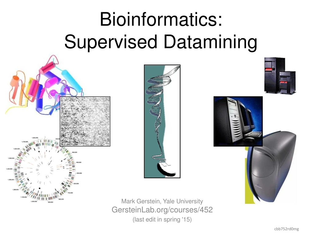
Bioinformatics: Supervised Datamining. Mark Gerstein, Yale University GersteinLab.org /courses/452 (last edit in spring '15). cbb752rd0mg. Supervised Learning. Given: training data The input objects (usually represented as vectors) – x, y values The labels – colors

E N D
Bioinformatics:Supervised Datamining Mark Gerstein, Yale UniversityGersteinLab.org/courses/452 (last edit in spring '15) cbb752rd0mg
Supervised Learning • Given: training data • The input objects (usually represented as vectors) – x, y values • The labels – colors • Define: a function that determines the labels given the input objects • Use the function to predict the labels of new objects Criminisi, Shotton, and Konukoglu Microsoft Technical Report 2011
Distinctions in Supervised Learning • Regression vs Classification • Regression: labels are quantitative • Classification: labels are categorical • Regularized vs Un-regularized • Regularized: penalize model complexity to avoid over-fitting • Un-regularized: no penalty on model complexity • Parametric vs Non-parametric • Parametric: an explicit parametric model is assumed • Non-parametric: otherwise • Ensemble vs Non-ensemble • Ensemble: combines multiple models • Non-ensemble: a single model
Arrange data in a tabulated form, each row representing an example and each column representing a feature, including the dependent experimental quantity to be predicted.
Decision Trees • Classify data by asking questions that divide data in subgroups • Keep asking questions until subgroups become homogenous • Use tree of questions to make predictions • Example: Is a picture taken inside or outside? Criminisi, Shotton, and Konukoglu Microsoft Technical Report 2011
What makes a good rule? • Want resulting groups to be as homogenous as possible Rule 2 Rule 1 All groups still 50/50 Unhelpful rule 2/3 Groups homogenous Good rule Nando de Freitas 2012 University of British Columbia CPSC 340
Quantifying the value of rules • Decrease in inhomogeneity • Most popular metric: Information theoretic entropy • Use frequency of classifier characteristic within group as probability • Minimize entropy to achieve homogenous group S =
Algorithm • For each characteristic: • Split into subgroups based on each possible value of characteristic • Choose rule from characteristic that maximizes decrease in inhomogeneity • For each subgroup: • if (inhomogeneity < threshold): • Stop • else: • Restart rule search (recursion)
Analysis of the Suitability of 500 M. thermo. proteins to find optimal sequences purification Retrospective Decision Trees [Bertone et al. NAR (‘01)]
Retrospective Decision TreesNomenclature 356 total Not Expressible Express-ible Has a hydrophobic stretch? (Y/N) [Bertone et al. NAR (‘01)]
Effect of Scaling (adapted from ref?) cbb752rd0mg
Extensions of Decision Trees • Decision Trees method is very sensitive to noise in data • Random forests is an ensemble of decision trees, and is much more effective.
Decision boundaries:SVM v Tree v Nearest NBR (a) A support vector machine (SVM) forms an affine decision surface (a straight line in the case of two dimensions) in the original feature space or a vector space defined by the similarity matrix (the kernel), to separate the positive and negative examples and maximize the distance of it from the closest training examples (the support vectors, those with a perpendicular line from the decision surface drawn). It predicts the label of a genomic region based on its direction from the decision surface. In the case a kernel is used, the decision surface in the original feature space could be highly non-linear. (b) A basic decision tree uses feature-parallel decision surfaces to repeatedly partition the feature space, and predicts the label of a genomic region based on the partition it falls within. (c) The one-nearest neighbor (1-NN) method predicts the label of a genomic region based on the label of its closest labeled example. In all three cases, the areas predicted to be positive and negative are indicated by the red and green background colors, respectively. [Yip et al. Genome Biology 2013 14:205 doi:10.1186/gb-2013-14-5-205]
Fisher discriminant analysis • Use the training set to reveal the structure of class distribution by seeking a linear combination • y = w1x1 + w2x2 + ... + wnxn which maximizes the ratio of the separation of the class means to the sum of each class variance (within class variance). This linear combination is called the first linear discriminant or first canonical variate. Classification of a future case is then determined by choosing the nearest class in the space of the first linear discriminant and significant subsequent discriminants, which maximally separate the class means and are constrained to be uncorrelated with previous ones. Solution of 1st variate cbb752rd0mg
Support Vector Machines • A very powerful tool for classifications • Example Applications: • Text categorization • Image classification • Spam email recognition, etc • It has also been successfully applied in many biological problems: • Disease diagnosis • Automatic genome functional annotation • Prediction of protein-protein interactions • and more…
Example: Leukemia patient classification ALL: acute lymphoblastic leukemia AML: acute myeloid leukemia William S Nobel. What is a support vector machine? Nature Biotechnology. 2006
A simple line suffices to separate the expression profiles of ALL and AML William S Nobel. What is a support vector machine? Nature Biotechnology. 2006
In the case of more than two genes, a line generalizes to a plane or “hyperplane”. • For generality, we refer to them all as “hyperplane” William S Nobel. What is a support vector machine? Nature Biotechnology. 2006
Is there a “best” line? William S Nobel. What is a support vector machine? Nature Biotechnology. 2006
The maximum margin hyperplane William S Nobel. What is a support vector machine? Nature Biotechnology. 2006
Denote each data point as (xi, yi) • xi is a vector of the expression profiles • yi = -1 or 1, which labels the class • A hyperplane can be represented as: w*x + b = 0 • The margin-width equals to: http://en.wikipedia.org/wiki/Support_vector_machine
Find a hyperplane such that: • No data points fall between the lines and • The margin 2/||w|| is maximized • Mathematically, • Minimizew,b 1/2 ||w||2, subject to: • for yi = 1, • for yi = -1, • Combining them, for any i, • The solution expresses w as a linear combination of the xi • So far, we have been assuming that the data points from two classes are always easily linearly separable. But that’s not always the case http://en.wikipedia.org/wiki/Support_vector_machine
What if… William S Nobel. What is a support vector machine? Nature Biotechnology. 2006
Allow a few anomalous data points William S Nobel. What is a support vector machine? Nature Biotechnology. 2006
The soft-margin SVM • subject to, for any i, • Si are the slack variables • C controls the number of tolerated misclassifications (It's effectively a regularization parameter on model complexity) • A small C would allow more misclassifications • A large C would discourage misclassifications • Note that even when the data points are linearly separable, one can still introduce the slack variables to pursue a larger separation margin http://en.wikipedia.org/wiki/Support_vector_machine cbb752rd0mg
Yes (by a 1D-hyperplane = dot) • Are linear separating hyperplanes enough? NO William S Nobel. What is a support vector machine? Nature Biotechnology. 2006
Transform (xi) into (xi, xi2) William S Nobel. What is a support vector machine? Nature Biotechnology. 2006
Non-linear SVM • In some cases (e.g. the above example), even soft-margin cannot solve the non-separable problem • Generally speaking, we can apply some function to the original data points so that different classes become linearly separable (maybe with the help of soft-margin) • In the above example, the function is f(x) = (x, x2) • The most import trick in SVM: to allow for the transformation, we only need to define the “kernel function”, • The above example essentially uses a polynomial kernel
Math behind the “kernel trick” • In optimization theory, a constrained optimization problem can be formulated into its dual problem (the original problem is called primal problem) • The dual formulation of SVM can be expressed as: • , subject to • The “Kernel”: , can be replaced by more sophisticated kernels: Complicated!
“Support vector machine”, where does the name come from? • The xi for which αi > 0 are called support vectors • They fall between or right on the separating margins from http://cbio.ensmp.fr/~jvert/talks/110401mines/mines.pdf
Key idea in the Kernel Trick • Original SVM optimization for refining the hyperplane parameters w & b in terms of a linear combination of xi can be replaced by a different optimization problem using "Lagrange multipliers" ai • One only optimizes using the product of xi*xj, now expressing the solution in terms of ai which are non-zero for xi that function as support vectors • In a non-linear SVM xi*xj is replaced by f(xi)*f(xj), so you don't need to know f(xi) itself only the product • This is further formalized in the kernel trick where f(xi)*f(xj) is just replaced by k(xi, xj). That is, one only has to know the “distance” between xi & xj in the high-dimensional space -- not their actual representation
Two commonly used kernels (and there are more) • Polynomial kernel: • a = 1 (inhomogeneous) or 0 (homogenous) • d controls the degree of polynomial and henceforth the flexibility of the classifier • degenerates to linear kernel when a = 0 and d = 1 • Gaussian kernel: • σ controls the width of the Gaussian and plays a similar role as d in the polynomial kernels
Questions for practitioners: Which kernel to use? How to choose parameters? • Trial and error • Cross-validation • High-degree kernels always fit the training data well, but at increased risks of over-fitting, i.e. the classifier will not generalize to new data points • One needs to find a balance between classification accuracy on the training data and regularity of the kernel (not allowing the kernel to be too flexible)
A low-degree kernel (left) and an over-fitting high-degree kernel (right) William S Nobel. What is a support vector machine? Nature Biotechnology. 2006
More about kernels • With kernels, non-vector data can be easily handled – we only need to define the kernel function between two objects • Examples of non-vector biological data include: DNA and protein sequences (“string kernels”), nodes in metabolic or protein-protein interaction networks, microscopy images, etc • Allows for combining different types of data naturally – define kernels on different data types and combine them with simple algebra cbb752rd0mg
Large C Small C Intermediate C http://cbio.ensmp.fr/~jvert/talks/110401mines/mines.pdf
The parameter C has a similar role • Small C will make few classification errors on the training data • But this may not generalize to the testing data • Large C pursues a large separating margin at the expenses of some classification errors on the training data. • The accuracy more likely to generalize to testing data cbb752rd0mg
Semi-supervised Methods • Supervised & Unsupervised: Can you combine them? YES • RHS (c) shows modifying the optimum decision boundary in (a) by "clustering" of unlabeled points [Yip et al. Genome Biol. ('13)] Supervised, unsupervised and semi-supervised learning. (a) In supervised learning, the model (blue line) is learned based on the positive and negative training examples, and the genomic region without a known class label (purple circle) is classified as positive according to the model. (b) In unsupervised learning, all examples are unlabeled, and they are grouped according to the data distribution. (c) In semi-supervised learning, information of both labeled and unlabeled examples is used to learn the parameters of the model. In this illustration, a purely supervised model (dashed blue line) classifies the purple object as negative, while a semi-supervised model that avoids cutting at regions with a high density of genomic regions (solid blue line) classifies it as positive.