Download
1 / 55
570 likes | 872 Views
PRICE DISCOVERY IN SPOT and FUTURE HARD COMMODITY MARKETS. Isabel Figuerola-Ferretti Jesus Gonzalo Universidad Carlos III de Madrid Business Department and Economic Department Preliminary October 2006. Trading Places Movie. We are going to talk about …. Introduction Theoretical Model

E N D
PRICE DISCOVERY IN SPOT and FUTURE HARD COMMODITY MARKETS Isabel Figuerola-Ferretti Jesus Gonzalo Universidad Carlos III de Madrid Business Department and Economic Department Preliminary October 2006
We are going to talk about … • Introduction • Theoretical Model • Econometric Implementation (GG P-T decomposition) • Data • Results • Conclusions
Price Discovery • The process by which future and cash markets attempt to identify permanent changes in transaction prices. • The essence of the price discovery function of future markets hinges on whether new information is reflected first in changed future prices or changed cash prices (Hoffman 1932).
Contribution • We separately quantify the relative contribution of future and spot prices to the revelation of the underlying fundamentals. • We demonstrate that for those metals with a liquid futures market the future price is more important in the price discovery process. • The Gonzalo-Granger decomposition allows us to do this more robustly than in Habroucks alternative way.
Why these commodity markets? • Commodities are traded in highly developed future markets. • In the metals sector 90% of the transactions take place in the forward/future markets. • The LME quoted price is the world wide reference price and the common. • It is important to quantify the price discovery role of metals futures.
Literature Review 1Literature on price discovery • Garbade, K. D. & Silver W. L. (1983). Price movements and price discovery in futures and cash markets. Review of Economics and Statistics. 65, 289-297. • Hasbrouck, J. 1995. One security, many markets: Determining the contributions to price discovery. Journal of Finance 50, 1175-1199. • Harris F., McInish T. H. Shoeshmith G. L. Wood R. A. (1995) Cointegration, Error Correction, and Price Discovery on Informationally Linked Security Markets. Journal of Financial and Quantitative Analysis. 30, 563-579
Literature Review 2:Price discovery metrics • Gonzalo, J. Granger C. W. J 1995. Estimation of common long-memory components in cointegrated systems. Journal of Business and Economic Statistics 13, 27-36. • Hasbrouck, J. 1995. One security, many markets: Determining the contributions to price discovery. Journal of Finance 50, 1175-1199
Literature Review 3Comparing the two metrics of price discoverySpecial Issue Journal of Financial Markets 2002 • Baillie R., Goffrey G., Tse Y., Zabobina T. 2002. Price discovery and common factor models. • Harris F. H., McInish T. H., Wood R. A. 2002. Security price adjustment across exchanges: an investigation of common factor components for Dow stocks. • Hasbrouck, J. 2002. Stalking the “efficient price” in market microstructure specifications: an overview. Leathan Bruce N. (2002). Some desiredata for the measurement of price discovery across markets. • De Jong, Frank (2002). Measures and contributions to price discovery: a comparison.
Theoretical Model: Garbade and Silber 1983Equilibrium with infinitely elastic supply of arbitrageAssumptions: • No taxes or transaction cost • No limitations on borrowing • No cost other than financing to storing a long cash market position • No limitations on short sale of the commodity in the spot market • The interest rate is flat and stationary at continuously compounded rate of r per unit time.
Theoretical Model: Garbade and Silver 1983 • Return of investing S0 € in the spot market • Alternatively investing S0 in a risk free asset and at the same time taking a long position in the future market (delivery in one year) produces the return
Theoretical Model: Garbade and Silver 1983 • Under the previous assumptions so • Taking logs, at time t the equilibrium with infinitely elastic supply of arbitrage is
Theoretical Model: Garbade and Silver 1983 where St and Ft are in logs, and tt is the number of days to the first delivery date of the underlying commodity (in our case, 15 months). • The previous assumptions imply that the supply of arbitrage services will be infinitely elastic whenever eq (1) is violated (1)
Theoretical Model: Garbade and Silver 1983 Equilibrium with finitely elastic supply of arbitrage services • Lets define a cash-equivalent future price • To describe the interaction between cash and future prices we must first specify the behavior of agents in the marketplace. • There are Ns participants in spot market. • There are Nf participants in futures market. • Ei,t is the endowment of the ith participant immediately prior to period t. • rit is the reservation price at which that participant is willing to hold the endowment Ei,t. • Elasticity of demand, the same for all participants.
Theoretical Model: Garbade and Silver 1983 Equilibrium with finitely elastic supply of arbitrage services • Demand schedule of ith participant in spot market where A is the elasticity of demand • Aggregate cash market demand schedule of arbitrageurs in period t where H is the elasticity of cash market demand by arbitrageurs. It is finite when the arbitrage transactions of buying in the cash market and selling the futures contract or vice-versa are not riskless
Theoretical Model: Garbade and Silver 1983 • The cash market will clear at the value of St that solves • The future market will clear at the value of Ft such that
Theoretical Model: Garbade and Silver 1983 Equilibrium with finitely elastic supply of arbitrage services • Solving the clearing market conditions we get • If there is no arbitrage H=0 • If H=∞
Theoretical Model: Garbade and Silver 1983 Dynamic price relationships • To derive dynamic price relationships, we need a description of the evolution of reservation prices.
Theoretical Model: Garbade and Silver 1983 • And the mean reservation price
Theoretical Model: Garbade and Silver 1983 Dynamic price relationships: VAR model • When H=0, prices are independent random walks • When H=∞ prices, will follow a common random walk (ets=etf ) • When 0<H<∞: • If Futures market dominate • If Cash markets dominate Mensures the importance of future markets relative to cash markets
Theoretical Model: Garbade and Silver 1983 VECM Representation The ratio is used to measure the importance of future market relative to the cash market in the price discovery process
Theoretical Model: Garbade and Silver 1983 • Alternatively substituting with k=rt
Theoretical Model: Garbade and Silver 1983 Incorporating Mean Backwardation/Contango
The ‘Theory’ of Normal Backwardation • Normal backwardation is the most commonly accepted “driver” of commodity future returns • “Normal backwardation” is a long-only risk premium “explanation” for futures returns • Keynes coined the term in 1923 • It provides the justification for long-only commodity futures indices • Keynes on Normal Backwardation “If supply and demand are balanced, the spot price must exceed the forward price by the amount which the producer is ready to sacrifice in order to “hedge” himself, i.e., to avoid the risk of price fluctuations during his production period. Thus in normal conditions the spot price exceeds the forward price, i.e., there is a backwardation. In other words, the normal supply price on the spot includes remuneration for the risk of price fluctuations during the period of production, whilst the forward price excludes this.” A Treatise on Money: Volume II, page 143
Backwardation refers to futures prices that decline with time to maturity • Contango refers to futures prices that rise with time to maturity Backwardation Nearby Futures Contract Contango Note: commodity price term structure as of May 30th, 2004
Theoretical Model: Garbade and Silver 1983 VECM with Mean Backwardation/Contango
Econometric Implementation • We use the Gonzalo-Granger (GG) methodology as opposed to Hasbrouck´s because it is robust to the presence of correlations in the error terms (et). • This is important for commodity price data with daily frequency. • Both techniques impose a minimum structure in the dynamics of the price series.
Metodology: the GG Permanent-Transitory P-T decomposition where
The steps are… 1) Perform unit root test on price levels 2) Estimate the VECM model 3) Test the rank of cointegration r 4) Estimate by finding the first r eigenvectors of the following eigenvalue problem 5) Estimate the α vector by finding the last n-r eigenvectors of the following eigenvalue problem
The steps are… 6) Test the H0: 7) Test the H0α = (1,0) and α = (0,1) 8) Set up the PT decomposition
Data • Daily spot and future (15 months) for Al, Cu, Ni, Pb, Sn, Zi, quoted in the LME. • Sample January 1990- July 2006. • Source Ecowin. • Copper: historically most important contract traded in LME. Aluminium took over in terms of volume in 1997. • Aluminium and Nickel trading introduced in 1979.
Conclusions and implications • For those metals with most liquid future markets the future price is the major contributor to the revelation of the common factor. • Producers and consumers should rely on the LME future price to make their production and consumption decisions. • The LME future price changes lead price changes in cash markets more often than the reverse. • Future and spot prices are cointegrated implying that it is not possible to make profits in the long run trading futures and taking positions in the underlying commodity