Download
1 / 18
180 likes | 278 Views
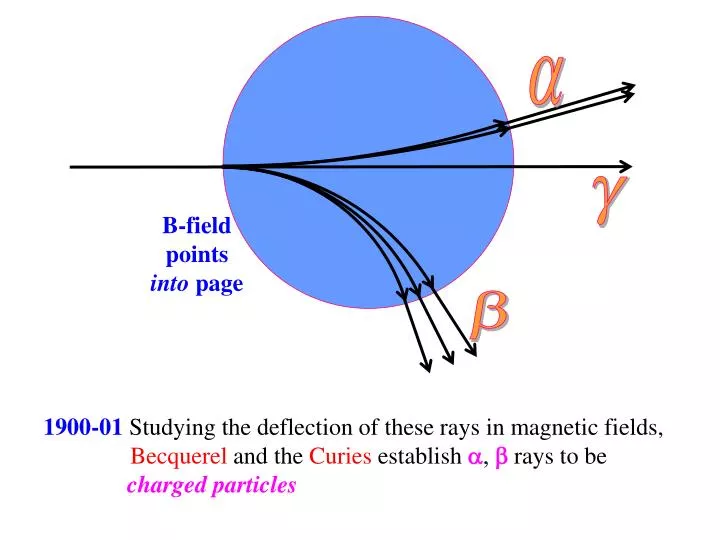
a. g. B-field points into page. b. 1900-01 Studying the deflection of these rays in magnetic fields, Becquerel and the Curies establish rays to be charged particles. 1900-01 Using the procedure developed by J.J. Thomson in 1887

E N D
a g B-field points into page b 1900-01 Studying the deflection of these rays in magnetic fields, Becquerel and the Curies establish rays to be charged particles
1900-01 Using the procedure developed by J.J. Thomson in 1887 Becquerel determined the ratio of charge q to mass m for : q/m = 1.76×10¹¹ coulombs/kilogram identical to the electron! : q/m = 4.8×10⁷ coulombs/kilogram 4000 times smaller!
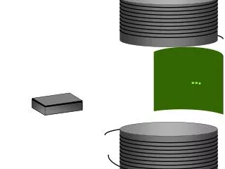
Noting helium gas often found trapped in samples of radioactive minerals, Rutherford speculated that particles might be doubly ionized Helium atoms (He++) 1906-1909Rutherford and T.D.Royds develop their “alpha mousetrap” to collect alpha particles and show this yields a gas with the spectral emission lines of helium! Discharge Tube Thin-walled (0.01 mm) glass tube to vacuum pump & Mercury supply Radium or Radon gas Mercury
Status of particle physics early 20th century Electron J.J.Thomson 1898 nucleus ( proton) Ernest Rutherford 1908-09 a Henri Becquerel 1896 Ernest Rutherford 1899 b g P. Villard 1900 X-rays Wilhelm Roentgen 1895
Periodic Table of the Elements 26 27 28 Fe Co Ni 55.86 58.93 58.71 Atomic “weight” values averaged over all isotopes in the proportion they naturally occur.
C 6 Through lead, ~1/4 of the elements come in “single species” Isotopes are chemically identical (not separable by any chemical means) but are physically different (mass) The “last” 11 naturally occurring elements (Lead Uranium) recur in 3 principal “radioactive series.” Z=82 92
92U23890Th234 91Pa234 92U234 92U23490Th230 88Ra226 86Rn222 84Po218 82Pb214 82Pb21483Bi214 84Po214 82Pb210 82Pb21083Bi210 84Po210 82Pb206 “Uranium I” 4.5109 years U238 “Uranium II” 2.5105 years U234 “Radium B” radioactive Pb214 “Radium G” stable Pb206
Chemically separating the lead from various minerals (which suggested their origin) and comparing their masses: Thorite (thorium with traces if uranium and lead) 208 amu Pitchblende (containing uranium mineral and lead) 206 amu “ordinary” lead deposits are chiefly207 amu
Masses are given in atomic mass units (amu) based on 6C12 = 12.000000
Mass of bare hydrogen nucleus: 1.00727 amu Mass of electron: 0.000549 amu
number of protons number of neutrons
Starting from the defining relation of a Fourier transform: -i k g'(x) g(x)= e+ikx f(x) we can integrate this “by parts” f(x) is bounded oscillates in the complex plane over-all amplitude is damped at ±
And so, specifically for a normal distribution:f(x)=e-x2/22 differentiating: from the relation just derived: Let’s Fourier transform THIS statement i.e., apply: on both sides! 1 2 ~ ~ ~ F'(k)e-ikxdk 1 2 ~ ei(k-k)xdx ~ (k – k)
1 2 ~ ei(k-k)xdx ~ (k – k) ~ selecting out k=k k k ' ' rewriting as: dk' dk' ' 0 0
Fourier transforms of one another Gaussian distribution about the origin Now, since: we expect: Both are of the form of a Gaussian! x k 1/
x k 1 or giving physical interpretation to the new variable x px h