Download
1 / 36
360 likes | 517 Views
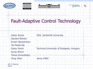
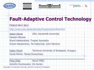
Fault-Adaptive Control Technology. Gabor Karsai Gautam Biswas Sriram Narasimhan Tal Pasternak Gabor Peceli Gyula Simon Tamas Kovacshazy Feng Zhao. ISIS, Vanderbilt University Technical University of Budapest, Hungary Xerox PARC. Objective. Develop and demonstrate FACT tool suite

E N D
Fault-Adaptive Control Technology Gabor Karsai Gautam Biswas Sriram Narasimhan Tal Pasternak Gabor Peceli Gyula Simon Tamas Kovacshazy Feng Zhao ISIS, Vanderbilt University Technical University of Budapest, Hungary Xerox PARC
Objective • Develop and demonstrate FACT tool suite • Components: • Modeling approach • Hybrid Diagnosis and Mode Identification System • Discrete Diagnosis and Mode Identification System • Dynamic Control Synthesis System • Transient Management System
Model-based Approach • Design-time and run-time activities are separated • Technology target: run-time SW Modeling Environment • Run-time Environment • Hybrid/Discrete Diagnostics • Controller selection • Transient management • Run-time platform (OCP) Model Database
Run-time System Architecture Monitor/ Hybrid Controller Diagnostics Library Active Model Failure Propagation Controller Diagnostics Selector Embedded Models Fault Detector Transient Manager Hybrid Observer Reconfigurable Monitoring and Control Reconfiguration System Controller Tools/components are model-based
Modeling language summary • System [plant] models • Physical components and assemblies • Aspects: • Structure: hierarchy and interconnectivity • Bond graph: quantitative/discrete nominal behavior, discrepancies • Local failures: failure modes, discrepancies,alarms • Failure propagations: causal chain of events • Failure models • Fine-grain: parametric failures in terms of bond-graph parameters • Large-grain: (discrete) failure modes and their functional effects (discrepancies) • Multi-modal behavior • Switched junctions in the bond graph model • Discrete modes in failure propagation graphs • Component types and system instances
Modeling language summary • Functional models • Modes contain Capabilities that reference Parameters in Components • Controller models • Hierarchical signal flow blocks • TBD: • Sensor/actuator interfaces • Controller characterization • Conditions for using a controller architecture
Continuous behavior is interspersed with discontinuities Discontinuities attributed to supervisory control and reconfiguration (fast switching) modeling abstractions (parameter & time-scale) Modeling language based on hybrid bond graphs (Jour. Franklin Inst. ‘97) Bond graphs for energy-based modeling of continuous behavior Switching junctions model controller and autonomous jumps systematic principles: piecewise linearization around operating points & derive transition conditions (CDC’99, HS’00) Plant modeling: Nominal behaviorDynamic Physical Systems
V1 Tank 1 Tank 2 Tank 3 V5 Sf2 Sf1 h1 h2 h3 R23n H4 H3 R12n H1 H2 V2 V3 V4 V6 R1 R2 R23v R12v 15 20 5 12 13 17 1 2 6 21 9 24 Sf1 Sf2 11 0 0 1 0 18 10 18 8 15 3 22 14 12 16 17 1,2,3,5,7,8: 4 11 16 23 6: R1 ON soni soffi OFF Plant modeling: Nominal behaviorExample Hybrid system: Three tank model of a Fuel System hi = level of fluid in Tank i Hi = height of connecting pipe R12v R23v 4: ON 14 7 h1 <H1 and h2<H2 h1H1 or h2H2 C3 C1 C2 13 OFF R12n R23n R2 ON h3 <H3 and h4<H4 h3H3 or h4H4 6 controlled junctions (1,2,3,5,7,8) 2 autonomous junctions (4,6) OFF
Application example: Fuel System Control for Fighter/Attack Aircraft • Problems: • Maintain fuel flow to the engines • Maintain A/C center of gravity • Affected by modes of operation: attack, cruise, • take-off, and landing • Compensate for component degradations and failures
Simplified Fuel System Schematics Wing Tank One Side Only Pump Feed Tank Load (Engine) Transfer Tank Pump Pump FM Detailed Model of AC Pump
1 1 R Rp4 Pump BG Fragment Pump BG Fragment Hybrid Bond Graph Model (Simplified Fuel System) I m1 R R1 I m2 Bond Graph Fragment: AC Pump a 2 5 7 n TF 1 3 4 6 8 Sf 1 0 1 MGY Controlled Junction Level Control Valve C CF I mp3 C CTR I mp1 R Rp4 Pump BG Fragment 1 0 0 1 0 R RLoad R Rp1 R Rp2 I mp2 R Rp3 1 C CW Fuel System BG: one side (valves – controlled junctions not shown) 0
Plant modeling: Nominal behaviorUsing the Hybrid Bond-Graph Hybrid Bond-graph Model Hybrid Observer Continuous observer A uk yk System Generation B z-1 C Hybrid Automata Generation Xk+1 xk m1 m2 Hybrid Automata Model m3 Mode switching logic
Plant modeling: Nominal behaviorImplementation of the hybrid observer On-line Hybrid Observer Embedded Hybrid Bond-graph Model Not necessary to pre-calculate all the modes, only the immediate follow-up modes are needed. Generate Current State-Space Model (A,B,C,D) High-level Mode (Switch settings) Mode change Detector Calculate: transition conditions, next states Recalculate Extended Kalman Filter uk,yk Xk Implement continuous + switching behavior Extended Kalman Filter
V1 Tank 1 Tank 2 Tank 3 V5 Sf2 Sf1 h1 h2 h3 R23n H4 H3 R12n H1 H2 V2 V3 V4 V6 R1 R2 R23v R12v Plant modeling: Nominal behaviorHybrid Observer: Tracking tank levels through mode changes h1 Mode 1: 0 t 10: Filling tanks v1, v3, & v4 open, v2, v5, & v6: closed h2 Mode 2: 10 t 20: Draining tanks v2, v3, v4, & v6 open, v1, & v5: closed Mode 3: 20 t : Tank 3 isolated v3 open, all others: closed : actual measurement : predicted measurement h3
FDI for Continuous Dynamic SystemsHybrid Scheme u y Plant - Nominal Parameters Observer and mode detector ŷ Hybrid models Fault Parameters mi progressive monitoring hypothesis refinement hypothesis generation Symbol generation Fault detection [Binary decision] r fh fh’ Parameter Estimation Diagnosis models Fault Isolation u = input vector, y = measured output vector, ŷ = predicted output using plant model, r = y – ŷ, residual vector, r= derived residualsmi= current mode, fh = fault hypotheses
Step 1 Step 2 Step 0 Qualitative diagnosis results Diagnosis results Measured variables e10 and f3 under fault conditions For more details: see (i) Mosterman and Biswas, IEEE SMC’99 & (ii) Manders, Narasimhan, Biswas, & Mosterman, Safeprocess 2000.
FDI for Continuous Dynamic Systems Quantitative Analysis: Fault Refinement,Degradations fh’ fh True Fault (C1) Other hypothesis (R12) Multiple Fault Observers
Failure Mode Discrepancy D +Alarm Sensor Time Interval Discrete Fault ModelsTimed Failure Propagation Graph
Discrete Fault ModelsGraphical Representation in GME • Propagation Attributes: • Time delay • Likelihood
Discrete Fault ModelsResearch Issues: Managing complexity in models • Locality: • Some phenomenon are not local (e.g. fire in the engine) or are a composite of local phenomena • To provide useful information the diagnosis must trace failures to individual components • Failure Modes are attributes of components • Hierarchy • For scalability it is important that the model accommodates diagnosis with different resolution • An FPG at one level will often incorporate Failure Modes of components at a lower level
Discrete Fault ModelsResearch Issues: Semantics of models • Failure Mode: • A condition of a component, which manifests in abnormal behavior. • Structural defect: parameter deviation • Failure modeled as “input” • Discrepancy: • An abnormal change in system state • Transition into abnormal state • Normal state, but abnormal transition • Fault Propagation: • Ordering of events • Where an event is a region in the extended system state space • Input x State x Next State
Discrete Fault ModelsResearch Issues: Expressing Constraints and Interactions • Incompatibility • When symptoms (or causes) can not co-occur (stuck_open stuck_closed) • Additivity • When the combination of effects produces an extra effect (primary and backup fail) • Cancellation • When effects negate, decrease, or mask each other
Discrete Fault ModelsResearch Issues: TFPG, FSM and Diagnostics • A model of a system as a timed (non-deterministic) Finite State Automata provides sufficient information to draw the full TFPG • Diagnosis can be performed using a partial TFPG model of the system
Discrete Fault ModelsResearch Issues: Implementing the Discrete Diagnostics • Extended Relational Algebra • Relational Algebra is used in databases to manipulate relations • Extended Relational Algebra allows nested relations • This allows to model logical constraints involving arbitrary logical expressions • Role • Discrete fault models as FSM-s • The complex state transition function of FSM-s can be represented using the Extended Relational Algebra and OBDD-s as the physical data structure
FlowController FC V FS P Flow Sensor Valve Pipe Discrete Fault ModelsRelating an FPG to FSM • Component Digraph • A link represents the fact that the faulty operation of the source component results in the faulty operation of the destination component • A Transition Event represents the cause and nature of the change: <triggering event, current state, next state> • Failure Propagation Graph links each transition event to its immediate successor. Only failure trajectories are represented
Discrete Fault Models Diagnosis using Extended Relational Models Contents of the hypothesis set: • State (Which nodes are we “in”) • Failure modes (Which got us “here”) Previously Hypothesized Set of Alarm Instances Previously Hypothesized Set of Failure Modes All combinations Any Set of Failure Modes Next Hypothesized Set of Alarm Instances Set of Failure Mode Instances Ringing Alarms
Discrete Fault Models Summary • Extended Relational Models offer a general formalism to express causality relations between failures and their symptoms, as well as constraints, interactions and composition • Extended Relational Models can also represent ordering of transition events in a dynamic system • Failure Propagation Graphs have been disambiguated by redefining them with a precise mapping to the Extended Relational Model See MSc thesis of Tal Pasternak on ISIS website
Towards an OCP implementation:Model-based software generation • Software models: • Controllers • Datatypes • Architectures
Plans • Vanderbilt/ISIS • Improve modeling language • Finish implementing Hybrid Diagnostics • Develop controller selection component • Fuel system example • Integration with OCP • Technical University of Budapest • Transient management techniques • Controller examples • Xerox/PARC • Data processing for fault detection