Download
1 / 39
400 likes | 765 Views
Logistic Regression. Chapter 8. Aims. When and Why do we Use Logistic Regression ? Binary Multinomial Theory Behind Logistic Regression Assessing the Model Assessing predictors Things that can go Wrong Interpreting Logistic Regression. When And Why.

E N D
Logistic Regression Chapter 8
Aims • When and Why do we Use Logistic Regression? • Binary • Multinomial • Theory Behind Logistic Regression • Assessing the Model • Assessing predictors • Things that can go Wrong • Interpreting Logistic Regression
When And Why • To predict an outcome variable that is categorical from one or more categorical or continuous predictor variables. • Used because having a categorical outcome variable violates the assumption of linearity in normal regression.
With One Predictor • Outcome • We predict the probability of the outcome occurring • b0 and b0 • Can be thought of in much the same way as multiple regression • Note the normal regression equation forms part of the logistic regression equation
With Several Predictor • Outcome • We still predict the probability of the outcome occurring • Differences • Note the multiple regression equation forms part of the logistic regression equation • This part of the equation expands to accommodate additional predictors
Assessing the Model • The Log-likelihood statistic • Analogous to the residual sum of squares in multiple regression • It is an indicator of how much unexplained information there is after the model has been fitted. • Large values indicate poorly fitting statistical models.
Assessing Changes in Models • It’s possible to calculate a log-likelihood for different models and to compare these models by looking at the difference between their log-likelihoods.
Assessing Predictors: The Wald Statistic • Similar to t-statistic in Regression. • Tests the null hypothesis that b = 0. • Is biased when b is large. • Better to look at Likelihood-ratio statistics.
Assessing Predictors: The Odds Ratio or Exp(b) • Indicates the change in odds resulting from a unit change in the predictor. • OR > 1: Predictor , Probability of outcome occurring . • OR < 1: Predictor , Probability of outcome occurring .
Methods of Regression • Forced Entry: All variables entered simultaneously. • Hierarchical: Variables entered in blocks. • Blocks should be based on past research, or theory being tested. Good Method. • Stepwise: Variables entered on the basis of statistical criteria (i.e. relative contribution to predicting outcome). • Should be used only for exploratory analysis.
Things That Can go Wrong • Assumptions from Linear Regression: • Linearity • Independence of Errors • Multicollinearity • Unique Problems • Incomplete Information • Complete Separation • Overdispersion
Incomplete Information From the Predictors • Categorical Predictors: • Predicting cancer from smoking and eating tomatoes. • We don’t know what happens when nonsmokers eat tomatoes because we have no data in this cell of the design. • Continuous variables • Will your sample contain a to include an 80 year old, highly anxious, Buddhist left-handed cricket player?
Complete Separation • When the outcome variable can be perfectly predicted. • E.g. predicting whether someone is a burglar or your teenage son or your cat based on weight. • Weight is a perfect predictor of cat/burglar unless you have a very fat cat indeed!
Overdispersion • Overdispersion is where the variance is larger than expected from the model. • This can be caused by violating the assumption of independence. • This problem makes the standard errors too small!
An Example • Predictors of a treatment intervention. • Participants • 113 adults with a medical problem • Outcome: • Cured (1) or not cured (0). • Predictors: • Intervention: intervention or no treatment. • Duration: the number of days before treatment that the patient had the problem.
Click Categorical Click First, then Change. See p 279 Identify any categorical Covariates (Predictors). With a categorical predictor with more than 2 categories you should use either the highest number to code your control category, then select last for your indicator contrast. In this data set 1 is cured, 0 not cured (our control category, therefore we select first as control, see p 279.
Enter Interaction Term(s) You can specify main effects and interactions. Highlight both predictors, then click the >a*b> If you don’t have previous literature, choose Stepwise Forward LR LR is Likelihood Ratio
Option Settings for Logistic Regression Hosmer-Lemeshow assesses how well the model fits the data. Look for outliers +/- 2 SD Request the 95% CI for the odds ratio (odds of Y occurring)
Output for Step 0, Constant Only Initially the model will always select the option with the highest frequency, in this case it selects the intervention (treated). Large values for -2 Log Likelihood (-2 LL) indicate a poor fitting model. The -2 LL will get smaller as the fit improves.
Example of How to Write the Logistic Regression Equation from Coefficients Using the constant only the model above predicts a 57% probability of Y occurring.
Equation for Step 1 See p 288 for an Example of using equation to compute Odds ratio. We can say that the odds of a patient who is treated being cured are 3.41 times higher than those of a patient who is not treated, with a 95% CI of 1.561 to 7.480. The important thing about this confidence interval is that it doesn’t cross 1 (both values are greater than 1). This is important because values greater than 1 mean that as the predictor variable(s) increase, so do the odds of (in this case) being cured. Values less than 1 mean the opposite: as the predictor increases, the odds of being cured decreases.
Output: Step 1 Removing Intervention from the model would have a significant effect on the predictive ability of the model, in other words, it would be very bad to remove it.
Classification Plot Further away from .5 is better. The .5 line represents a coin toss you have a 50/50 chance. If the model fits the data, then the histogram should show all of the cases for which the event has occurred on the right hand side (C), and all the cases for which the event hasn’t occurred on the left hand side (N). This model is better at predicting cured cases than it is for non cured cases, as the non cured cases are closer to the .5 line.
Choose Analyze – Reports – Case Summaries Use the Case Summaries function to create a table of the first 15 cases showing the values of Cured, Intervention, Duration, the predicted probability (PRE_1) and the predicted group membership (PGR_1).
Summary • The overall fit of the final model is shown by the −2 log-likelihood statistic. • If the significance of the chi-square statistic is less than .05, then the model is a significant fit of the data. • Check the table labelled Variables in the equation to see which variables significantly predict the outcome. • Use the odds ratio, Exp(B), for interpretation. • OR > 1, then as the predictor increases, the odds of the outcome occurring increase. • OR < 1, then as the predictor increases, the odds of the outcome occurring decrease. • The confidence interval of the OR should not cross 1! • Check the table labelled Variables not in the equation to see which variables did not significantly predict the outcome.
Multinomial logistic regression • Logistic regression to predict membership of more than two categories. • It (basically) works in the same way as binary logistic regression. • The analysis breaks the outcome variable down into a series of comparisons between two categories. • E.g., if you have three outcome categories (A, B and C), then the analysis will consist of two comparisons that you choose: • Compare everything against your first category (e.g. A vs. B and A vs. C), • Or your last category (e.g. A vs. C and B vs. C), • Or a custom category (e.g. B vs. A and B vs. C). • The important parts of the analysis and output are much the same as we have just seen for binary logistic regression
I may not be Fred Flintstone … • How successful are chat-up lines? • The chat-up lines used by 348 men and 672 women in a night-club were recorded. • Outcome: • Whether the chat-up line resulted in one of the following three events: • The person got no response or the recipient walked away, • The person obtained the recipient’s phone number, • The person left the night-club with the recipient. • Predictors: • The content of the chat-up lines were rated for: • Funniness (0 = not funny at all, 10 = the funniest thing that I have ever heard) • Sexuality (0 = no sexual content at all, 10 = very sexually direct) • Moral vales (0 = the chat-up line does not reflect good characteristics, 10 = the chat-up line is very indicative of good characteristics). • Gender of recipient
Interpretation • Good_Mate: Whether the chat-up line showed signs of good moral fibre significantly predicted whether you got a phone number or no response/walked away, b = 0.13, Wald χ2(1) = 6.02, p < .05. • Funny: Whether the chat-up line was funny did not significantly predict whether you got a phone number or no response, b = 0.14, Wald χ2(1) = 1.60, p > .05. • Gender: The gender of the person being chatted up significantly predicted whether they gave out their phone number or gave no response, b = −1.65, Wald χ2(1) = 4.27, p < .05. • Sex: The sexual content of the chat-up line significantly predicted whether you got a phone number or no response/walked away, b = 0.28, Wald χ2(1) = 9.59, p < .01. • Funny×Gender: The success of funny chat-up lines depended on whether they were delivered to a man or a woman because in interaction these variables predicted whether or not you got a phone number, b = 0.49, Wald χ2(1) = 12.37, p < .001. • Sex×Gender: The success of chat-up lines with sexual content depended on whether they were delivered to a man or a woman because in interaction these variables predicted whether or not you got a phone number, b = −0.35, Wald χ2(1) = 10.82, p < .01.
Interpretation • Good_Mate: Whether the chat-up line showed signs of good moral fibre did not significantly predict whether you went home with the date or got a slap in the face, b = 0.13, Wald χ2(1) = 2.42, p > .05. • Funny: Whether the chat-up line was funny significantly predicted whether you went home with the date or no response, b = 0.32, Wald χ2(1) = 6.46, p < .05. • Gender: The gender of the person being chatted up significantly predicted whether they went home with the person or gave no response, b = −5.63, Wald χ2(1) = 17.93, p < .001. • Sex: The sexual content of the chat-up line significantly predicted whether you went home with the date or got a slap in the face, b = 0.42, Wald χ2(1) = 11.68, p < .01. • Funny×Gender: The success of funny chat-up lines depended on whether they were delivered to a man or a woman because in interaction these variables predicted whether or not you went home with the date, b = 1.17, Wald χ2(1) = 34.63, p < .001. • Sex×Gender: The success of chat-up lines with sexual content depended on whether they were delivered to a man or a woman because in interaction these variables predicted whether or not you went home with the date, b = −0.48, Wald χ2(1) = 8.51, p < .01.