Download
1 / 42
420 likes | 542 Views
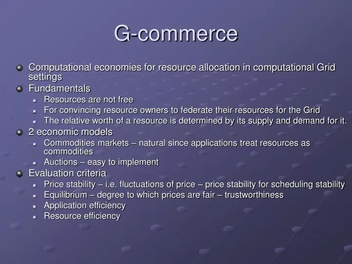
G-commerce. Computational economies for resource allocation in computational Grid settings Fundamentals Resources are not free For convincing resource owners to federate their resources for the Grid The relative worth of a resource is determined by its supply and demand for it.

E N D
G-commerce • Computational economies for resource allocation in computational Grid settings • Fundamentals • Resources are not free • For convincing resource owners to federate their resources for the Grid • The relative worth of a resource is determined by its supply and demand for it. • 2 economic models • Commodities markets – natural since applications treat resources as commodities • Auctions – easy to implement • Evaluation criteria • Price stability – i.e. fluctuations of price – price stability for scheduling stability • Equilibrium – degree to which prices are fair – trustworthiness • Application efficiency • Resource efficiency
Commodity Markets and Auctions • Commodity Markets • A third-party (market) sets a price for resources and asks producers and consumers willing to agree to that price • The participants engage in transactions • Based on unsatisfied demands and supplies, new prices are set • Consumers don’t ask for specific commodity but chooses one out of many equivalents • An attempt is made to satisfy all bidders and sellers at a given price • Auctions • A third-party (auctioneer) collects resources and bids • Highest bidder gets a resource per auction round • Prices are set based on bids • Process repeated for other resources • Consumers ask for specific commodities • One bidder and one seller satisfied at a given price
Producer and Consumer Models • Producer model • CPU • Disk • Producer will sell all of its remaining capacities at a given price point if it will turn a profit with respect to average profit over time • Consumers and jobs • Consumers are given initial budget and periodic allowances • Budgets are refreshed at periodic intervals • Consumers and producers agree on a price and during each simulated minute, the producer’s revenue is incremented and consumer’s budget is decremented • Consumers will place demand only if the capable_rate is >= avg_rate
Producer and Consumer Models • Summary • Producers consider long term profit and past performance when deciding to sell • Consumers are given periodic budget replenishments and spend opportunistically • Consumers introduce work load in bulk at the beginning of each simulated day, and randomly throughout the day
Commodities market and dynamic pricing • Pricing methodology for market economy • Pricing methodology should produce a system of price adjustments which bring about market equilibrium • Market economy is a system involving producers, consumers, several commodities, supply and demand functions for each commodity determined by the set of market prices for various commodities • A unique equilibrium price is guaranteed to exist in this framework
Commodities • Commodity prices represented by price vector, p. • zj - Excess demand for the jth commodity, i.e. demand minus supply • Each zj is a function of all prices pi • Smale’s theorem: an equilibrium point with p* such that excess demand vector z(p*) = 0 exists
Commodities Market Formulation • A nxn matrix of partial derivatives • Smale’s method: With λ same sign as determinant of Dz(p), economic equilibrium can be obtained by - • Lamda = 1 ; Euler discretization at positive values of t; reduces the process toNewton Raphson method for solving z(p) = 0 • Approximate each excess demand function zi by a polynomial in p1,p2,…pn • Use partial derivates of the polynomials • High polynomial of degree 17 was used • This procedure is called first bank of G method
Auctions • When an application desires multiple commodities, it places multiple bids on multiple auctions and obtains some of the resources • It expends currency on the obtained resources while it waits for other resources • Auctions are highly unreliable in terms of pricing and ability to obtain resource – leads to poor scheduling decisions
Simulations of auctions • At each time step, CPU and disk producers submit their unused slots, minimum selling price (average profit / slot) to auctioneers • Consumers define bid prices based on demand functions and bid on each commodity needed by their jobs • Highest bidding customer gets commodity • Price of the commodity – average of commodity’s minimum selling price and consumer’s bid price
Simulation experiments • 2 scenarios • Under-demand – producers can adequately support consumers • Over-demand – consumers wish to buy more resources than available • Simulation setting • Under-demand • 100 consumers to use 100 CPUs and disks • Each consumer submitted random number of jobs (between 1 to 100) at every simulated day break • 10% chance of submitting new job every time unit • Over-demand • 500 of the same consumers
Market equilibrium – commodity markets: Illustration of equilibrium by Smale’s method
Market equilibrium - auctions • Variance in prices due to different prices paid by different bidders increase over time – i.e. price becomes less stable over time • Spikes in workload are not reflected in price. • Disk prices are identical even though they are plentiful in number – should be low-priced.
Market equilibrium - Summary • Smale’s method is appropriate for modeling hypothetical Grid market • First bank of G reasonable and implementable approximation • Auctioneering attractive from implementation standpoint • But does not produce stable pricing or market equilibrium • Grid resource allocation decisions based on auctioneering lack fairness • Commodities market formulation perform better from the standpoint of Grid as a whole • Over-demand case performed similar to under-demand
Efficiency results • Utilization of resources from supplier standpoint • Number of jobs completed / time unit from consumer standpoint
Other Pricing Models • Posted Price Model • Special offers to motivate users to utilize unused slots • Bargaining Model • Tender/contract-net model • Bid-based proportional resource sharing model • Used in cooperative resource sharing environments • Share-holders model • When users are both service providers and consumers • Monopoly
An Incentive-based Grid Scheduling • Resource Consumers • Job length, job deadline • Resource Providers • Capability, unit price and job queue • Scheduling objective • Provide QoS to consumers. Highly successful (without missing deadline) execution rate of job • Reasonable profit for providers. Fair allocation of benefits, i.e. the profit of every provider is proportional to its investment or cost
Overall Design • Peer-2-peer grid • Step 1 – a consumer submits job announcement, broadcast to all providers • Step 2 - Provider estimates whether it is able to meet deadline. Yes- provider sends a bid containing the charge for the job • Step 3 - Consumer processes all the bids and chooses the provider with the least charge. Sends job • Step 4 - Provider queues it, executes and sends results
Job Competing Algorithm for Step 2 • How a provider bids. Job competing algorithm • After a provider has sent its bid to previous job (unconfirmed job), when a job announcement comes for a new job, should it consider the previous job for deciding on whether to bid for the new job? • Parameter α, conservation degree • α = 0, aggressive. Don’t consider unconfirmed jobs when estimating whether it will meet a new job deadline • α = 1, conservative. Consider unconfirmed jobs when estimating whether it will meet a new job deadline
Job competing algorithm • Invoked when a producer receives a bid • Step 1 – provider estimates whether it is able to meet the job deadline • place0 to placen – n+1 possible places for inserting a new job Jn+1 • Available time – when all jobs in queue will be completed • T = (deadline – execution time) latest time by which job has to start to meet deadline
Algorithm • If can_meet = true; go to step 2
Job Competent Algorithm • Step 2 – provider fixes a price for the job • Step 3 • provider sends the price as the bid • Inserts in insert_place with a probability CD • If job offer doesn’t come after some time, deletes it from the queue
Heuristic Local Scheduling Algorithm for step 3 • If CD is not 1 (conservative), jobs may miss deadline • Hence, need for a punishment mechanism to producers for missing deadlines • Hence providers need mechanisms to minimize loss • One way – try all permutations of job ordering and choose the one with minimum penalty – NP complete • A heuristic algorithm that is invoked every time a producer is offered a job that it has not kept in the queue
Price Adjustments • Initially, a market price for a commodity is fixed • When a provider enters the grid, gets this market price and uses it as initial unit price • Every time a provider is offered a job or deletes an unconfirmed job, invokes the price adjustment algorithm
Algorithm • Offered_job_length – aggregated length of jobs offered to the provider • Total_job_length – aggregated length of jobs whose announcements have been received by the producer
Simulation Setup • 20 consumers, 80 producers • Fixed values for • Average lengths of jobs • Average of capabilities of providers • λ,α,β • Market price • Different system loads • CD – 0, 0.5, 1
Incentive of Consumers • Based on 2 metrics • A job fails because all providers decide not to bid
Results • Failure rate increases with higher system load and when the producers are more conservative • Deadline missing rate increases with higher system and when the producers are more aggressive
Results • Deadline missing rate has much lesser impact. Hence conservative is not good
Incentive for Providers • Penalty of providers increases as CD decreases • For total profit, tradeoff CD of 0.5 is good
Fairness • Should be close to 1. • Intuitively, aggressive competing ensures fairness; items are mostly sold at low base price
Game-Theory Based Pricing Strategy • Pricing strategy implemented between job allocator and nodes using game theoretic framework • The 2 players are job allocator and nodes • They play incomplete information, alternating-offers, noncooperative, bargaining game to decide on • Price per unit resource • Percentage of bandwidth that can be used on the link between job allocator and nodes • If there are n nodes, a JA plays a game with each of the n nodes to form vectors of price and percentage bandwidth
Incomplete Information • Two players have no idea of each other’s reserved valuations • JA • Maximum offered price • Minimum bandwidth percentage • Node • Minimum expected price • Maximum bandwidth percentage • Both can make surplus or profit and try to reach a mutually beneficial arrangement
Rules for JA • Rule 1 – at each step of the game, both players choose the alternative earning them highest expected price • Expected utility = [(reserved valuation of JA – offered price) + (offered percentage of bandwidth – minimum percentage)] x probability(offered price, percentage of bandwidth offered) • Probability – that the tuple will be accepted by the opponent
Rules for JA • Rule 2 – on rejection of an offer, JA and the node reduce the probability • Reduction decreases as alternatives come closer to their reserved valuations • Rule 3 – demands of JA and the node are decreased over time • e-z{w,m}t denotes discount rates of JA and node. Thus • Expected utility = [(reserved valuation of JA – offered price) + (offered percentage of bandwidth – minimum percentage)] x probability(offered price, percentage of bandwidth offered) x e-zwt
Utility Functions for Pricing Strategy for JA • If JA accepts the current offer, its expected utility is:
Utility Functions for Pricing Strategy for JA • If JA rejects the opponent’s offer and breaks down from the game:
Utility Functions for Pricing Strategy for JA • In case of counteroffer:
References / Sources / Credits • Wolski, R., Plank, J., Brevik, J, and Bryan, T., G-Commerce: Market Formulations Controlling Resource Allocation on the Computational Grid (PDF), IPDPS 01, March, 2001. • Buyya et. al. Economic Models for Resource Management and Scheduling in Grid Computing. Concurrency and Computation. Practice and Experience. 2002. 14: 1507-1542. • GridIS: An Incentive Based Grid Scheduling. Xiao et. al. IPDPS 2005 • A Game Theory-Based Pricing Strategy to Support Single/Multiclass Job Allocation Schemes for Bandwidth-Constrained Distributed Computing Systems. Ghosh et. al. TPDS 2007.
Differences • In commodity markets, an attempt is made to satisfy all bidders and sellers at a given price • In auctions, one bidder and seller is satisfied at a given price