Download

1 / 22
260 likes | 478 Views
Bresenham’s Line Algorithm. The Problem (cont…). What happens when we try to draw this on a pixel based display?. How do we choose which pixels to turn on?.

E N D
The Problem (cont…) • What happens when we try to draw this on a pixel based display? • How do we choose which pixels to turn on?
In Bresenham’s line drawing algorithm the incremental integer calculations are used to scan convert the lines, so that, the circles and the other curves can be displayed. ? ? ? ?
.The next sample positions can be plotted either at (3,2) or (3,3) ? ? (3,3) ? ? ? (3,2) (2,2)
Advantages of DDA • It calculates the pixel positions faster than the calculations performed by using the equation y=mx +b. • Multiplication is eliminated as the x and y increments are used to determine the position of the next pixel on a line
Disadvantages of DDA • The rounding and floating point operations are time consuming. • The round-off error which results in each successive addition leads to the drift in pixel position, already calculated
For lines with positive slope m<1 • The pixel positions on line can be identified by doing sampling at unit x intervals. • The process of sampling begins from the pixel position (X0,Y0) and proceeds by plotting the pixels whose ‘Y’ value is nearest to the line path. • If the pixel to be displayed occurs at a position (Xk, Yk) then the next pixel is either at (Xk+1,Yk) or (Xk+1,Yk+1) i.e, (3,2) or (3,3) • The ‘Y’ coordinate at the pixel position Xk+1 can be obtained from • Y=m(Xk+1)+b . . . . . . . . . . ……. eq 1
the separation between (Xk+1,Yk) and (Xk+1,Y) is d1 and the separation between (Xk+1,Y) and (Xk+1, Yk+1) is d2 then • d1 = y – yk and • d2 = (Yk+1) – Y (Xk+1, yk+1) (Xk, yk+1) . d2 P0 d1 (Xk, yk) (Xk+1,yk)
Y=m(Xk+1)+b . . . . . . . ……. eq 1 • d1=y – yk • d1=m(xk+1)+b – Yk ( from eqn (1) …..( 2) • And d2= (Yk+1) – Y • =(YK+1) – [m(Xk+1)+b] • =(YK+1) – m(Xk+1) – b …….(3) • The difference is given as • d1-d2 = • = m(Xk+1)+b-Yk-[(Yk+1)-m(Xk+1)-b] • =m(Xk+1)+b-Yk-(Yk+1)+m(Xk+1)+b • d1-d2 = 2m(Xk+1)-2Yk+2b – 1 ………(4)
Contd.. • A decision parameter Pk can be obtained by substituting m= dy/dx in equation 4 • d1 – d2 = 2m(Xk+1)-2Yk+2b – 1 • = 2 dy/dx (Xk+1) – 2Yk + 2b – 1 • = 2 dy(Xk+1)-2 dx.Yk + 2b.dx -dx • dx • dx(d1-d2) = 2 dy(Xk+1)-2 dx.Yk + 2b.dx - dx • = 2 dyXk+2 dy-2 dx.Yk + 2b.dx -dx • = 2 dyXk- 2 dx.Yk + c • Where, dx(d1-d2) = Pk and • c= 2 dy+ dx(2b-1) • Pk = 2 dyXk- 2 dx.Yk + c . . . . . . . . . . . . . . . . . . . … …(5 ) • The value of c is constant and is independent of the pixel position. It can be deleted in the recursive calculations, of for Pk • if d1 < d2 (i.e, Yk is nearer to the line path than Yk+1) then, Pk is negative. • If Pk is –ve, a lower pixel (Yk)is plotted else, an upper pixel (Yk+1)is plotted. • At k+1 step, the value of Pk is given as • PK+1 = 2 dyXk+1- 2 dx.Yk+1 + c …………………………………..(6 ) (from 5)
M • Eq 6 – eq 5 • Pk+1 – Pk = (2 dyXk+1- 2 dx.Yk+1 + c ) - (2 dyXk+2 dx.Yk + c) • = 2dy(Xk+1-Xk ) – 2 dx(Yk+1 –Yk ) ………….(7) • Since Xk+1 = Xk +1 The eqn 7 becomes • Pk+1 – Pk = 2dy(Xk +1-Xk ) – 2 dx(Yk+1 –Yk ) • = 2dy - 2 dx(Yk+1 –Yk ) • Pk+1 = Pk + 2dy - 2 dx(Yk+1 –Yk ) ………………..( 8) • Where (Yk+1 – Yk) is either 0 or 1 based on the sign of Pk. • The starting parameter P0 at the pixel position (X0,Y0) is given as • P0 = 2dy – dx ………………………(9)
y=mx+c is the eq of line In col 2 the line is passing through x0+1 so the y value is given by y=m(x0+1)+c (green dot) Now we need to find out the values of d1 and d2 d1= y-y0 d2=(y0+1)-y d1=m(x0+1) – y0 and d2= (y0+1) - m(x0+1) d1-d2=[mx0+m – y0] - [(y0+1) - mx0-m] =mx0+m – y0 - y0-1 + mx0+m = 2mx0+2m –2y0-1 = 2mx0+2m –2mx0-1 (y=mx+c passes thr (x0, y0) so we can say y0=mx0+c) d1-d2 = 2mx0+2m –2mx0-1 d1-d2=2m-1 ( m= ∆y / ∆x) d1-d2 = 2∆y/ ∆x - 1 P0= 2∆y - ∆x Col 1 Col 2 (X0+1, y0+1) (X0, y0+1) d2 P0 d1 (X0, y0) (X0+1,y0) ∆x(d1-d2) = 2∆y - ∆x ∆x(d1-d2) = 2∆y - ∆x
Bresenham’s algorithm • Step 1: Enter the 2 end points for a line and store the left end point in (X0,Y0). • Step 2: Plot the first point be loading (X0,Y0) in the frame buffer. • Setp 3: determine the initial value of the decision parameter by calculating the constants dx, dy, 2dy and 2dy-2dx as • P0 = 2dy –dx • Step 4: for each Xk, conduct the following test, starting from k= 0 • If Pk <0, then the next point to be plotted is at (Xk+1, Yk) and • Pk+1 = Pk + 2dy • Else, the next point is (Xk+1, Yk+1) and • Pk+1 = Pk + 2dy –2dx (step 3) • Step 5: iterate through step (4) dx times.
Example • Let the given end points for the line be (30,20) and (40, 28) • M = dy = y2 – y1 = 28 – 20 = 8 • dx x2 – x1 40 – 30 = 10 • m = 0.8 • dy = 8 and dx = 10 • The initial decision parameter P0 is • P0 = 2dy – dx = 2(8) – 10 = 16 – 10 = 6 • P0 = 6 • The constants 2dy and 2dy-2dx are • 2dy = 2(8) = 16 2dy-2dx = 2(8)- 2(10) =16 – = 20 • 2dy = 162dy – 2dx = - 4
The starting point (x0, y0)=(30,20) and the successive pixel positions are given in the following table
End points (30,20) (40,28) • dx=x2-x1=40-30=10 dy= y2-y1=28-20=8 • P0=2dy-dx=2X8-10 = 6 >0 pt(31,21) • Pk+1= pk+2dy-2dx= 6+16-20 =2 >0 (32,22) • Pk+1=2+16-20 =-2 <0 (33,22) • Pk+1= pk+2dy =-2+16 = 14 >0 (34,23) • Pk+1= pk+2dy-2dx=14+16-20=10>0 (35,24) • Pk+1=10+16-20=6 >0 (36,25) • Pk+1= 6+16-20=2>0 (37,26) • Pk+1=2+16-20=-2 <0 (38,26) • Pk+1= pk+2dy=-2+16=14>0 (39,27) • Pk+1=pk+2dy-2dx= 14+16-20=10>0 (40,28)
In bresenham’s algorithm, if the positive slope of a line is greater than 1, the roles of x and y are interchanged. • For positive slope lines: • If the initial position of a line is the right end point, then both x and y are decremented as we move from right to left. • If d1 = d2 then always select the upper or the lowet candidate pixel. • For negative slope lines: • One coordinate increases and the other coordinate decreases. • Special cases: • the vertical lines dx = 0, horizontal lines dy = 0 and diagonal lines |dx| = |dy| can be directly loaded into the frame buffer.
Void LineBres( int x1, int y1, int x2, int y2) { int dx =abs(x2-x1), dy= abs(y2-y1) int p=2* dy- dx ; int x, y, Xend; // Xends is similar to steps in DDA If(x1>x2) { x=x2;y=y2;Xend=x1; } else { x=x1;y=y1;Xend=x2; } setPexel( x, y ); While( x < Xend) { x++; if( p < 0) p=p+2dy; else { y++; p=p+2dy-2dx; } setPixel(x,y); } // End While } //End LineBres
Advantages of Bresenham’s Alg. • It uses only integer calculations • So, it is faster than DDA