Evaluating Theoretical Models

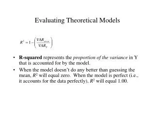
1. Evaluating Theoretical Models • R-squared represents the proportion of the variance in Y that is accounted for by the model. • When the model doesn’t do any better than guessing the mean, R2 will equal zero. When the model is perfect (i.e., it accounts for the data perfectly), R2 will equal 1.00.

2. Neat fact • When dealing with a simple linear model with one X, R2 is equal to the correlation of X and Y, squared. • Why? Keep in mind that R2 is in a standardized metric in virtue of having divided the error variance by the variance of Y. Previously, when working with standardized scores in simple linear regression equations, we found that the parameter b is equal to r. Since b is estimated via least-squares techniques, it is directly related to R2.

3. Why is R2 useful? • R2 is useful because it is a standard metric for interpreting model fit. • It doesn’t matter how large the variance of Y is because everything is evaluated relative to the variance of Y • Set end-points: 1 is perfect and 0 is as bad as a model can be.

4. Why is R2 useful? • Finally, and importantly, we can begin to compare the relative fit of alternative models • Why is this useful? • When we began our discussion of modeling, we noted that there are ways to estimate parameter values, assuming the basic model is correct. • Now, we can begin to address the question of whether the basic model is correct by studying the model’s R2 and comparing it to the R2 produced by competing models.

5. Example • Data Person x y 1 -2 -11.6 2 -1 -4.4 3 0 1.0 4 1 0.4 5 2 -3.6

6. Model with no x • The most basic model we can study is one in which Y-hat = My • Recall, that the predicted values yield a horizontal line centered at the mean of Y (-4 in this example)

7. Model with no x • The variance of Y is 18 (rounded) • The dotted lines here represent the error in prediction • If we square these errors, we find the average squared error to be approximately 18 • Thus, R2 for this model is 1-(18/18) or 0.

8. Model with linear term • Next, let’s see what happens if we study a linear model of form Y-hat = a + bX • The average squared error in this example is 10.07 • R2 is .44 (1 – (10/18)). The linear model accounts for 44% of the variance in Y.

9. Model with a quadratic term • Next, let’s see what happens if we study a model of form Y-hat = a + bX2 • The average squared error in this example is approximately 8. • R2 is .55 (1 – (8/18)). The quadratic model accounts for 55% of the variance in Y (11% more than the linear model).

10. Model with linear and quadratic terms • Next, let’s see what happens if we study a linear + quad model of form Y-hat = a + bX + cX2 • The average squared error in this case is about .10. • R2 is .99 (1 – (.10/18)). The linear + quadratic model accounts for 99% of the variance in Y (44% more than the quadratic model alone).

11. Summary of model comparisons • Summary of the fit statistics for the various models Model R2 No clue .00 Linear .44 Quadratic .55 Linear + Quad .99

12. Summary • So, it looks like the model that combines the linear and the quadratic terms is the best model, of the four that we studied. It accounts for the data almost perfectly (99% of the variance in Y was explained by the model) • Note that the model is imperfect • What does this mean? • Either the model is not the true representation of reality and some other model is needed • Maybe there is some imperfection in the data (which, of course, represents a flaw in the model, but maybe not one we care too much about)

13. Residual term • A combination of these two options is considered frequently. In fact, the basic linear model often contains a variable that explicitly represents the influence of variables not considered explicitly by one’s theory • This variable is often called the residual or error term, and is often denoted by the Greek symbol epsilon or the Roman letter E. The variance of the residual scores is identical to the proportion of variance in Y that is unexplained by the model. If the model is good, the residual variance will be very small.

14. Residual Term • DATA = MODEL + RESIDUAL

15. E is approximate