Download
1 / 47
490 likes | 639 Views
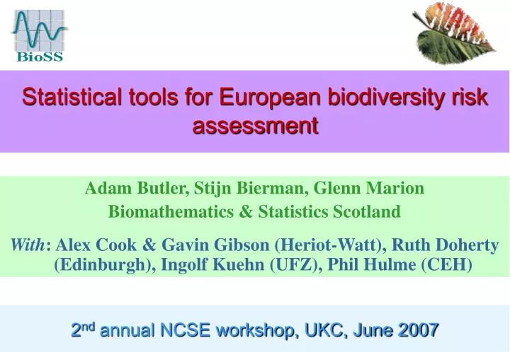
Statistical tools for European biodiversity risk assessment. Adam Butler, Stijn Bierman, Glenn Marion Biomathematics & Statistics Scotland With : Alex Cook & Gavin Gibson (Heriot-Watt), Ruth Doherty (Edinburgh), Ingolf Kuehn (UFZ), Phil Hulme (CEH). 2 nd annual NCSE workshop, UKC, June 2007.

E N D
Statistical tools for European biodiversity risk assessment Adam Butler, Stijn Bierman, Glenn Marion Biomathematics & Statistics Scotland With: Alex Cook & Gavin Gibson (Heriot-Watt), Ruth Doherty (Edinburgh), Ingolf Kuehn (UFZ), Phil Hulme (CEH) 2nd annual NCSE workshop, UKC, June 2007
The ALARM project • Assessing Large-scale risks to biodiversity with tested methods • Project of the 6th framework programme of the European Union • Runs from 2004-2009, involves 200+ scientists and social scientists, working in 67 organisations in 35 countries • Main website: www.alarmproject.net • BioSS is a partner, with three staff currently working on the project
Key objectives • Develop an integrated risk assessment for biodiversity in terrestrial and freshwater ecosystems at the European scale • Focus on four key pressures – climate change, invasive species, chemical pollution, pollinator loss – and their interactions • Contribute to the dissemination of scientific knowledge and to the development of evidence-based policy
Scenarios Assessments relate to six scenarios of climate & land use change • GRAS:deregulation, free trade, growth, globalization • BAMBU: “Business as might be usual” • SEDG: Sustainable European Development Goal • CUT: collapse of the thermohaline circulation • SEL: energy price shock, mass growth in biofuels • DEATH: global pandemic
The role of BioSS • Research-consultancy: develop & apply novel quantitative methods to support scientific research within ALARM • Training: Development of an online training course on statistical methods for environmental risk assessment • Dissemination: Contribute to the construction of a risk assessment toolkit for European biodiversity
Research themes 1 Statistical analysis of species atlas data 2 Quantification of uncertainty in complex mechanistic models 3 Elicitation of expert opinion regarding environmental risk
Species atlas data Galium pumilum (slender bedstraw) Mean annual temperature 1960-1990 (oC) Species atlas data record the presence/absence of species, for each cell on a regular grid – e.g. Florkart database of German vascular plants
Distribution of individual species • Atlas data are often used to analyze relationships between environmental variables & the spatial distribution of a particular species • Aim is often predictive: e.g. climate envelope modeling • Crude statistical analyses are based on multiple regression • Analyses should be modified to account for spatial autocorrelation & non-detection
Bierman, S.M., Wilson, I.J., Elston, D.A., Marion, G., Butler, A. & Kühn, I. (in preparation) Bayesian image restoration techniques to analyze species atlas data with spatially varying non-detection probabilities. Spatial autocorrelation Zi = I(species present in cell i) xi = covariates for cell i dij = distance between cells i and j Autologistic model (Augustin et al., 1996) Zi is a latent random variable
Bierman, S.M., Wilson, I.J., Elston, D.A., Marion, G., Butler, A. & Kühn, I. (in preparation) Bayesian image restoration techniques to analyze species atlas data with spatially varying non-detection probabilities. Non-recording yi = I(species recorded present in cell i) zi = I(species actually present in cell i); a latent random variable Mit =1 if Oit =1 Mit =0 or 1 if Oit = 0 set up Markov chain Monte Carlo sampler on Mit such that Oit = 0/1; Prior Likelihood Posterior
Detection effort Galium pumilum (slender bedstraw)
Distribution of functional traits Kühn, I., Bierman, S.M., Durka, W. & Klotz, S. (2006) Relating geographical variation in pollination types to environmental and spatial factors using novel statistical methods. New Phytologist, 172(1), 127-139. Pollination types in Germany
Spread of invasive species • Species atlas data for invasive species may also contain information on time of arrival, establishment or naturalization • We can, with care, use such data to draw inferences about the spatio-temporal spread of a species across a landscape, and thereby to assess the risks associated with future expansion • Need to deal with environmental heterogeneity: land use & climate
Spread of Giant Hogweed (Heracleum Mantegazzianum)Data : National Biodiversity Network By 1910
Spread of Giant Hogweed (Heracleum Mantegazzianum)Data : National Biodiversity Network By 1920
Spread of Giant Hogweed (Heracleum Mantegazzianum)Data : National Biodiversity Network By 1930
Spread of Giant Hogweed (Heracleum Mantegazzianum)Data : National Biodiversity Network By 1940
Spread of Giant Hogweed (Heracleum Mantegazzianum)Data : National Biodiversity Network By 1950
Spread of Giant Hogweed (Heracleum Mantegazzianum)Data : National Biodiversity Network By 1960
Spread of Giant Hogweed (Heracleum Mantegazzianum)Data : National Biodiversity Network By 1970
Spread of Giant Hogweed (Heracleum Mantegazzianum)Data : National Biodiversity Network By 1980
Spread of Giant Hogweed (Heracleum Mantegazzianum)Data : National Biodiversity Network By 1990
Spread of Giant Hogweed (Heracleum Mantegazzianum)Data : National Biodiversity Network By 2000
Cook, A., Marion, G., Butler, A. and Gibson, G. (2007). Bayesian inference for the spatio-temporal invasion of alien species. Bulletin of Mathematical Biology, in press. • Dispersal rate modelled using a symmetric power law kernel: • Arrival rate is treated as additive • Colonization rate • Dispersal modelled using symmetric power law kernel • Colonization suitability for each site a function of Land-cover & Climatic covariates • Key methodological challenge: estimate covariate effects dji = distance from cell i to cell j xi= covariates for cell i Ni = neighborhood of cell I Ti= year of colonization • Extend previous work by inclusion of “suitability”, S(xi)
Cook, A., Marion, G., Butler, A. and Gibson, G. (2007) Posterior mean Posterior mean Colonizationprobability: 10 year prediction Colonization suitability
Cook, A., Marion, G., Butler, A. and Gibson, G. (2007) Cumulative rate of colonization without covariates with covariates
Further work • Deal with inhomogeneities in the recording process: e.g. could analyse as three atlas surveys • Allow for decolonisation • Allow for time-varying covariates: e.g. land use change
Complex models • Complex mechanistic models provide a valuable tool for generating projections of large-scale environmental change • Models are typically deterministic, but with uncertain inputs (parameter values, initial values & boundary conditions) • Models are evaluated across a regular spatio-temporal lattice • Model outputs tend to exhibit systematic bias, e.g. because sub-gridscale processes are not represented
Doherty, R., Butler, A. & Marion, G. (in prep.) title to be decided • Use the Lund-Potsdam-Jena dynamic vegetation model to generate projected trends in global vegetation for the 21st century • Control run: use climate inputs provided by observational data • Other runs: inputs provided by simulations from one of nine General Circulation Models Scenario SRES A2 “A future world of very rapid economic growth, low population growth and rapid introduction of new and more efficient technology. Major underlying themes are economic and cultural convergence and capacity building, with a substantial reduction in regional differences in per capita income. In this world, people pursue personal wealth rather than environmental quality…”
Doherty, R., Butler, A. & Marion, G. (in prep.) title to be decided Global annual net primary productivity “Net primary production is the rateat which new biomass accrues in an ecosystem” (Wikipedia) Data: PCMDI (www-pcmdi.llnl.gov), CRU (www.cru.uea.ac.uk)
Statistical post-processing • Regression (Allen et al., 2002): x = mM mym + e • Hierarchical Bayesian modeling (Tebaldi et al., 2005): Model each of x and y1,…,y|M| as independent realisations of “reality”, which is a latent variable, • Bayesian model averaging (Raftery et al., 2005): f(x) = mM wm g(ym) g(ym) estimated from a simple statistical model ym = output from model mM x = corresponding data
Butler, A., Marion, G. & Doherty, R. (in prep.) Statistical averaging of long-term projections generated by a set of environmental models • Assign weights w1,…,w|M| ym = output from model mM x = corresponding data
Butler, A., Marion, G. & Doherty, R. (in prep.) Statistical averaging of long-term projections generated by a set of environmental models • Assign weights w1,…,w|M| • Calculate zm = ym - x ym = output from model mM x = corresponding data
Butler, A., Marion, G. & Doherty, R. (in prep.) Statistical averaging of long-term projections generated by a set of environmental models • Assign weights w1,…,w|M| • Calculate zm = ym – x • Fit a set of possible statistical models, hn(zm), where nN ym = output from model mM x = corresponding data
Butler, A., Marion, G. & Doherty, R. (in prep.) Statistical averaging of long-term projections generated by a set of environmental models • Assign weights w1,…,w|M| • Calculate zm = ym – x • Fit a set of possible statistical models, hn(zm), where nN • Apply a simple form Bayesian model averaging, gm(zm) = mM vn hn(zm), where vn exp(-BICn / 2) ym = output from model mM x = corresponding data
Butler, A., Marion, G. & Doherty, R. (in prep.) Statistical averaging of long-term projections generated by a set of environmental models • Assign weights w1,…,w|M| • Calculate zm = ym – x • Fit a set of possible statistical models, hn(zm), where nN • Apply a simple form Bayesian model averaging, gm(zm) = nN vn hn(zm), where vn exp(-BICn / 2) • Apply a second level of model averaging, f(x)= mM wm gm(ym – x) ym = output from model mM x = corresponding data
Doherty, R., Butler, A. & Marion, G. (in prep.) title to be decided
Doherty, R., Butler, A. & Marion, G. (in prep.) title to be decided
Statistical methods: an overview Single deterministic model SACCO: Statistical Analysis of Computer Code Output Single stochastic model ABC: Approximate Bayesian Computation Multiple deterministic models Statistical post-processing
SACCO methods R bundle: http://cran.r-project.org/src/contrib/Descriptions/BACCO.html Generate a set of ensembles,y(1),…, y(M) Emulation: construct a statistical model, (), which describes the relationship between inputs & outputs – a basis for interpolation Calibration (Kennedy & O’Hagan, 2001): relate output to reality, via x = () + () + e, where and are Gaussian processes y() = output from model given inputs x = corresponding data
ABC methods Assign informative prior distribution() to parameters Simulate from the prior, m ~ (), and then model, y(m) ~Y(m) Accept m if any only if D(y(m), x) < where D is a suitable distance metric and is small Samples from an approximation to the posterior of |x,Y Y() = output from model given inputs x = corresponding data
Integrated risk assessment • One of the key tasks of ALARM is to produce a risk assessment toolkit (RAT) for European biodiversity • The RAT requires us to link detailed, often quantitative, scientific assessments about risk with the requirements of policy-makers • This involves the integration of observational data, output from mechanistic models, and expert knowledge
Expert elicitation A process of representing expert beliefs and opinions about the properties of a system in the form of one or more probability distributions “The goal of elicitation, as we see it, is to make it as easy as possible for subject-matter experts to tell us what they believe, in probabilistic terms, while reducing how much they need to know about probability theory to do so…” (Kadane & Wolfson, 1998)
The elicitation process Kadane & Wolfson (1998), O’Hagan (1998) Elicit basic quantities: means, quantiles Produce a graphical representation Fit a statistical model Negative feedback Negative feedback Potential dangers Availability Overconfidence Anchoring Inconsistency Hindsight bias Principles Focus on observables Quantiles rather than moments Avoid tail probabilities Focus on prediction Interactive process
Threats to Bees • Within ALARM, we are assisting Koos Biesmeijer (Leeds) in using expert opinion to identify the primary cause of decline in threatened European bee species Potential threats Primary threat: species on UK red list Intrinsic factors Habitat loss Low densities Restricted range Native species dynamics Resource changes: Host plants Hosts (cleptoparasitic bees) Climate change