Download
1 / 49
490 likes | 600 Views
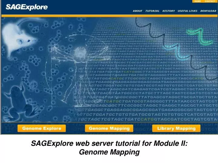
SAGExplore web server tutorial for Module II: Genome Mapping. II.- Genome Mapping Module: This module allows the user to map experimental tags against the genome.

E N D
SAGExplore web server tutorial for Module II: Genome Mapping
II.- Genome Mapping Module: This module allows the user to map experimental tags against the genome.
I.- Genome Mapping Module Form: The user must follow five sequential steps in this form. Online help with the relevant details is provided for each step.
Step 1: The user must select the organism of interest. Currently, only Saccharomyces cerevisiae is available. In the near future, other organisms will be added.
Step 2: The user must select the anchoring-tagging enzyme pair used in SAGE. Currently, only the pair NlaIII-BsmFI is available. In the near future, other enzyme pairs such as the one used in Long-SAGE will be added.
Step 3: The user must select the odds ratio used to assign the confidence classes to the different genomic tags. For details see: Malig, R., Varela, C., Agosin, E. and Melo, F. (2006) Accurate and unambiguous tag-to-gene mapping in SAGE by a hierarchical gene assignment procedure. BMC Bioinformatics, 7, 487-507.
Step 4: The user can choose to map the experimental tags against a subset of genomic tags upon a large amount of different features. For details see the help links or: Malig, R., Varela, C., Agosin, E. and Melo, F. (2006) Accurate and unambiguous tag-to-gene mapping in SAGE by a hierarchical gene assignment procedure. BMC Bioinformatics, 7, 487-507.
Step 5: The user must provide a list of experimental tags to map against the genome-based annotation of virtual or potential tags. A text file can be uploaded or the data directly pasted into the textarea. The input format is explained in the help link for this step. Full tag sequences must be provided (ie. including the CATG).
Pre-submit: Before submitting the query, the user can choose the number of rows to display per page and also how to sort the results.
Submit: The user is ready to submit the query to the server.
Query Results: The total number of records that matched the query are reported. Also, the total number of unmatched tags (NIDs or Non-Identified Tags) out of the total number of submitted tags is given.
Query Results: Only a fraction of the results is displayed. This option can be easily changed by selecting a different number of rows to display or the next button used to go to the next page.
Query Results: The full table can be downloaded as tab-delimited text (compressed file or tar.gzipped).
Query Results: Compressed files for download are kept for 5 hours at the server and then deleted. By clicking on the filename, the file is downloaded.
Query Results: Online help explaining the meaning of each column is obtained by left-clicking with the mouse over the column headers.
Query Results: By clicking over the standard gene name, a query to the Saccharomyces Genome Database is launched. Thus, the user can obtain a large amount of data about a given gene.
Query Results: By clicking over the systematic gene name, a query to the Saccharomyces Genome Database is launched. Thus, the user can obtain a large amount of data about a given gene.
SGD Query: An example of the results obtained when quering the Saccharomyces Genome Database by standard or systematic gene name.
Query Results: The genomic context where a tag matches can be obtained by clicking on this field.
Genomic Context: The selected tag is shown with a vertical arrow head.
Genomic Context: Gene names are linked to the Saccharomyces Genome Database.
Genomic Context: Keys of the graphical elements displayed above are provided.
Genomic Context: The fragment of the chromosome being displayed is specified.
Genomic Context: In this case corresponds to the 5’ end of the chromosome. The user can click on this graphical chromosome to select and display a different region.
Genomic Context: The chromosome scale in base pairs is also shown.
Genomic Context: The current chromosome number and size are given.
Genomic Context: The 5’ and 3’ positions of the chromosome fragment displayed are also shown.
Genomic Context: Clicking on the tag will display a pop-up window with several details about this tag. This pop-up window can also be launched from the main results table and thus it will be explained next from there.
Query Results: A record with several tag details can be obtained by clicking on this field.
Tag details: Many details about the tag are provided here. See the online help for an explanation of each field meaning.
Query Results: The genomic sequence context where the tag matches can be downloaded by clicking on this field.
Download Sequence: If the tag matches an ORF (as it is in this example), the transcript sequence is given. The 5’ and 3’ UTRs, the start and stop codons, and the tag sequence are all highlighted. If the tag matches an intergenic region, the 500 flanking nucleotides upstream and downstrem the tag are provided. In this case, neighbor elements such as UTRs from other genes are also highlighted if present.
Download Sequence: The FASTA header indicates the exact region of the sequence displayed.
Query Results: A query to the BLAST server at the NCBI is launched with the previosuly described sequence by clicking on this field. In the case of tags matching an intergenic region, this option is very useful to aid the process of gene discovery.
BLAST Query: A query to the BLAST server at the NCBI is automatically launched with the flanking sequence that contains the tag. In the case of intergenic tags, BLASTX is launched (this example). In the case of tags matching an ORF, BLASTP is used.
Query Results: The tag counts provided by the user are shown here (in case the user provided this information). In this case, the counts of three independent experiments were provided and shown.
Query Results: Each tag can have a label (if the user provided it), which is displayed in this field. This could be useful to highlight some specific tags of interest, or for example, to see the cluster group number of each tag. The user can provide any label here. This field is optional and can be empty (as it is this example case).
Query Results: An expression map with the counts of all the mapped tags onto the genome is available by following the highlighted button.
Expression Map: An expression map with the counts of all the mapped tags onto the genome is displayed. This is useful to detect transcriptionally active regions in a chromosome.
Expression Map: The user can select a single experimental condition or to display all of them simultaneously (as it is the case in this example). The ‘show’ button on the right must be clicked to make effective any change of parameters.
Expression Map: The user can select a range of expression level. Only the tags which counts belong to this expression range will be displayed. The ‘show’ button on the right must be clicked to make effective any change of parameters.
Expression Map: The user can select two types of scale for the Y axis of the graph: linear or logarithmic. The ‘show’ button on the right must be clicked to make effective any change of parameters.
Expression Map: The tags mapped are graphically shown in the chromosome.
Expression Map: The start and end coordinates of the chromosome fragment displayed are given. Also, in the chromosome, the selected region is highlighted. The graph below shows the counts of each tag for each experimental condition, as supplied by the user.
Expression Map: By clicking on a given tag count, several tag details are given in a pop-up window.
Tag details: Many details about the tag are provided here. See the online help for an explanation of each field meaning.
This is the end of the SAGExplore web server tutorial for Module II: Genome Mapping Any comments or inquiries, please contact us