Download
1 / 10
120 likes | 293 Views
HIERARCHICAL LINEAR MODELS. USED WITH NESTED DESIGNS IN EDUCATION, PSYCHOLOGY USES RANDOM FACTORS EXPECTED MEAN SQUARE THEORY COMBINES INFORMATION ACROSS LEVELS TO ESTIMATE VARIANCES, STANDARD ERRORS PRODUCES CORRECT STANDARD ERRORS FOR F-TESTS. TWO LEVEL ANOVA.

E N D
HIERARCHICAL LINEAR MODELS • USED WITH NESTED DESIGNS IN EDUCATION, PSYCHOLOGY • USES RANDOM FACTORS EXPECTED MEAN SQUARE THEORY • COMBINES INFORMATION ACROSS LEVELS TO ESTIMATE VARIANCES, STANDARD ERRORS • PRODUCES CORRECT STANDARD ERRORS FOR F-TESTS
TWO LEVEL ANOVA Student score = Class mean + Indiv. Error yij = Ci + pij Class mean = School mean + Class error Ci = S + eij yij = ( S + eij ) + pij Thus, student score has class variation in it, the effect of being in, and influencing a particular class.
TWO LEVEL ANOVA Correction to standard errors: SEcor = SE [ 1 + (nclus -1) ] , nclus = # students per class where = Intraclass correlation : var(class)/[var(class) + var(student)]
TWO LEVEL ANOVA SEcor = SE [ 1 + (nclus -1) ] , nclus = # students per class where = Intraclass correlation : Average (rclass) > rschool Example: SE = SD/ SQRT(nclus) = 2.236 let = .1, SD= 10, nclus = 20 SEcor = {10/4.472}[ 1+ (20-1)*.1] = 6.485
Y raverage= .5 School regression rschool = 0 X
ANCOVA and ATI for HLM • Dep. Variable: Popularity • Fixed effects: Pupil gender • Random effects: Teacher experience • Model: yij = b0j + b1j Gen + eij b0j = g00 + g01 Exp + u0j Intercepts b1j = g10 + g11 Exp + u1j Slopes
boys Popular I ty girls Class 1 Class 2 Teacher Experience
GLM ANALYSIS OF PREFERENCE AND AGGRESSION R-Square Coeff Var Root MSE mrat1 Mean 0.171843 20.13344 0.658391 3.270139 Source DF Type I SS Mean Square F Value Pr > F ovg 1 292.0628803 292.0628803 673.76 <.0001 agmean 1 0.2496626 0.2496626 0.58 0.4480 ovg*agmean 1 0.0163565 0.0163565 0.04 0.8460 Source DF Type III SS Mean Square F Value Pr > F ovg 1 21.83289074 21.83289074 50.37 <.0001 agmean 1 0.24986698 0.24986698 0.58 0.4478 ovg*agmean 1 0.01635649 0.01635649 0.04 0.8460 Standard Parameter Estimate Error t Value Pr > |t| Intercept 3.293216737 0.03268211 100.77 <.0001 ovg -1.521097692 0.21433132 -7.10 <.0001 agmean -0.124159266 0.16353429 -0.76 0.4478 ovg*agmean -0.199813164 1.02863958 -0.19 0.8460
HLM ANALYSIS OF PREFERENCE AND AGGRESSION Covariance Parameter Estimates Standard Z Cov Parm Subject Estimate Error Value Pr Z UN(1,1) cls 0.09404 0.01264 7.44 <.0001 INTERCEPT OVG UN(2,1) cls 0.03315 0.02609 1.27 0.2038 COV INT-SLOPE UN(2,2) cls 0.4096 0.1071 3.82 <.0001 SLOPE OVG Residual 0.3328 0.008725 38.15 <.0001 Type 3 Tests of Fixed Effects Num Den Effect DF DF F Value Pr > F OVG 1 163 37.39 <.0001 OVGMEAN(CLASS) 1 2920 5.06 0.0246 OVG*OVGMEAN 1 2920 0.01 0.9068
CLASSROOM 1 PREFERENCE CLASSROOM 2 CLASSROOM 5 CLASSROOM4 CLASSROOM 3 CLASSROOM MEAN AGGRESSION