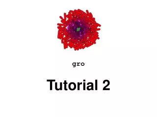
gro Tutorial 2
gro Tutorial 2. Functions. This line defines a function called “hill” that takes three arguments (v, k and x) and returns a simple calculation on those arguments. . include gro fun hill v k x . v * x / ( k + x ); print ( hill 1.0 1.0 1.0 ); print ( hill 1.0 1.0 2.0 );.

gro Tutorial 2
E N D
Presentation Transcript
Functions This line defines a function called “hill” that takes three arguments (v, k and x) and returns a simple calculation on those arguments. include gro fun hill v k x . v * x / ( k + x ); print ( hill 1.0 1.0 1.0 ); print ( hill 1.0 1.0 2.0 ); These two print statements print the value of the hill function applies to different arguments in the message window at the bottom of the . Note that these statements run upon loading the program, and before you click start. Try defining other functions. You can use an operators you like (+,-,*,^,/,%) as well as things like sqrt(x), sin(y), etc. Note that functions defined with “fun” expect their arguments separated by spaces not by commas. You can add parentheses as in hill (v+1) k (x/100) for example to disambiguate expressions. Read the documentation for more information. Internally defined functions like sin(x) or print() take their arguments, on the other hand, take arguments in parentheses as with, for example, matlab or C.
Use the Function in a Cell Program include gro fun hill v k x . v * x / ( k + x ); alpha := 1.0; km := 10.0; iptg := 1.0; program p() := { gfp := 0; rate ( hill alpha km iptg ) : { gfp := gfp + 1; } }; ecoli ( [], program p() );
Chemostat Mode include gro chemostat ( true ); fun hill v k x . v * x / ( k + x ); alpha := 1.0; km := 10.0; iptg := 1.0; program p() := { gfp := 0; rate ( hill alpha km iptg ) : { gfp := gfp + 1; } }; ecoli ( [], program p() ); Media flow Chemostat mode allows you to keep a more or less fixed population of cells in the simulation as long as you want.
Chemostat Size include gro chemostat ( true ); set ( "chemostat_width", 20 ); set ( "chemostat_height", 250 ); fun hill v k x . v * x / ( k + x ); alpha := 1.0; km := 10.0; iptg := 1.0; program p() := { gfp := 0; rate ( hill alpha km iptg ) : { gfp := gfp + 1; } }; ecoli ( [], program p() ); Media flow
include gro chemostat ( true ); fun hill v k x . v * x / ( k + x ); alpha := 1.0; km := 10.0; iptg := 1.0; program p() := { gfp := 0; rate ( hill alpha km iptg ) : { gfp := gfp + 1; } }; ecoli ( [], program p() ); program main() := { t := 0; true : { t := t + dt, iptg := 50 * ( 1 + sin(0.05*t) ), clear_messages ( 1 ), message ( 1, tostring(iptg) ) } }; main() Functions The special program main() is not associated with a cell. Instead, it is run once per timestep, and can be used to control the simulation. For example, here we are changing the level of iptg according to a sine wave. Note that iptg is a global variable, so it available to all of the cells and to the main function.
Compose Two Programs ... fp := fopen ( "/tmp/data.csv", "w" ); program report(period) := { t := 0; s := 0; needs gfp; true : { t := t + dt, s := s + dt } s >= period : { fprint ( fp, id, ", ", t, ", ", gfp/volume, "\n" ); s := 0; } }; program q() := p() + report(10) sharing gfp; ecoli ( [], program q() ); ... This program prints out the gfp/volume value of the corresponding cell. The new program q() is the composition of the old program p() from previous slides, and the new report program. You can use this report program with whatever program you want. gfp is shared between the two programs. It is the same variable. Note that the variables t and s in report(period) are not shared, and are thus not in the top level scope of q() – meaning that they don’t get cut in half when the cell divides.
In MATLAB… data=sortrows(load('data.csv')); maxid=max(data(:,1)); wave=[0:400;10*(1+sin(0.05*(0:400)))]'; plot(wave(:,1),wave(:,2)) hold on; hue=hsv(maxid+1); for i=0:maxid idx=find(data(:,1)==i); cellData=data(idx,2:3); plot(cellData(:,1),cellData(:,2),'Color',hue(i+1,:)) end; xlabel('time'); ylabel('gfp/vol');
In R… data = read.csv("data.csv",header=FALSE); maxid <- max(data$V1); plot(0:400,10*(1+sin(0.05*(0:400))),type="l",col="blue",xlab="time",ylab="gfp/vol") attach(data); for(i in 0:maxid) { tmp <- data[which(V1==i),]; T <- tmp$V2; GFP <- tmp$V3; lines(T,GFP,type="l",col=hsv(i/maxid)) } dev.copy(pdf,"example2_r.pdf") dev.off()
SimulationControl ... chemostat ( false ); ... program main() := { t := 0; true : { t := t + dt } t > 100 : { print ( iptg, ”, ", maptocells gfp/volume end ), iptg := iptg + 1, reset(), ecoli ( [], program p() ), start(), t := 0 } iptg > 10 : { stop() } }; You can use main to do a variety of other simulation manipulation. For example, you can start(), stop(), and reset() the simulation to do multiple experiments. Note that reset() deletes all the cells, so you need to add a new cell after calling it. This program grows cells for 100 simulated minutes, prints some data, resets the iptg level, and starts over.


