Download
1 / 45
490 likes | 1.2k Views
Cost Minimization. Molly W. Dahl Georgetown University Econ 101 – Spring 2009. Cost Minimization. A firm is a cost-minimizer if it produces a given output level y ³ 0 at smallest possible total cost.

E N D
Cost Minimization Molly W. Dahl Georgetown University Econ 101 – Spring 2009
Cost Minimization • A firm is a cost-minimizer if it produces a given output level y ³ 0 at smallest possible total cost. • When the firm faces given input prices w = (w1,w2,…,wn) the total cost function will be written as c(w1,…,wn,y).
The Cost-Minimization Problem • Consider a firm using two inputs to make one output. • The production function isy = f(x1,x2). • Take the output level y ³ 0 as given. • Given the input prices w1 and w2, the cost of an input bundle (x1,x2) is w1x1 + w2x2.
The Cost-Minimization Problem • For given w1, w2 and y, the firm’s cost-minimization problem is to solve subject to
The Cost-Minimization Problem • The levels x1*(w1,w2,y) and x1*(w1,w2,y) in the least-costly input bundle are the firm’s conditional factor demands for inputs 1 and 2. • The (smallest possible) total cost for producing y output units is therefore
Conditional Factor Demands • Given w1, w2 and y, how is the least costly input bundle located? • And how is the total cost function computed?
Iso-cost Lines • A curve that contains all of the input bundles that cost the same amount is an iso-cost curve. • E.g., given w1 and w2, the $100 iso-cost line has the equation
Iso-cost Lines • Generally, given w1 and w2, the equation of the $c iso-cost line isRearranging… • Slope is - w1/w2.
Iso-cost Lines x2 Slopes = -w1/w2. c” º w1x1+w2x2 c’ º w1x1+w2x2 c’ < c” x1
The y’-Output Unit Isoquant x2 All input bundles yielding y’ unitsof output. Which is the cheapest? f(x1,x2) º y’ x1
The Cost-Minimization Problem x2 All input bundles yielding y’ unitsof output. Which is the cheapest? x2* f(x1,x2) º y’ x1* x1
The Cost-Minimization Problem At an interior cost-min input bundle:(a) and(b) slope of isocost = slope of isoquant x2 x2* f(x1,x2) º y’ x1* x1
The Cost-Minimization Problem At an interior cost-min input bundle:(a) and(b) slope of isocost = slope of isoquant; i.e. x2 x2* f(x1,x2) º y’ x1* x1
A Cobb-Douglas Ex. of Cost Min. • A firm’s Cobb-Douglas production function is • Input prices are w1 and w2. • What are the firm’s conditional factor demand functions?
A Cobb-Douglas Ex. of Cost Min. At the input bundle (x1*,x2*) which minimizesthe cost of producing y output units: (a)(b) and
A Cobb-Douglas Ex. of Cost Min. (a) (b)
A Cobb-Douglas Ex. of Cost Min. (a) (b) From (b),
A Cobb-Douglas Ex. of Cost Min. (a) (b) From (b), Now substitute into (a) to get
A Cobb-Douglas Ex. of Cost Min. (a) (b) From (b), Now substitute into (a) to get So is the firm’s conditionaldemand for input 1.
A Cobb-Douglas Ex. of Cost Min. Since and is the firm’s conditional demand for input 2.
A Cobb-Douglas Ex. of Cost Min. So the cheapest input bundle yielding y output units is
A Cobb-Douglas Ex. of Cost Min. So the firm’s total cost function is
A Cobb-Douglas Ex. of Cost Min. So the firm’s total cost function is
A Cobb-Douglas Ex. of Cost Min. So the firm’s total cost function is
A Perfect Complements Ex.: Cost Min. • The firm’s production function is • Input prices w1 and w2 are given. • What are the firm’s conditional demands for inputs 1 and 2? • What is the firm’s total cost function?
A Perfect Complements Ex.: Cost Min. x2 4x1 = x2 min{4x1,x2} º y’ x1
A Perfect Complements Ex.: Cost Min. x2 Where is the least costly input bundle yielding y’ output units? 4x1 = x2 min{4x1,x2} º y’ x1
A Perfect Complements Ex.: Cost Min. x2 Where is the least costly input bundle yielding y’ output units? 4x1 = x2 min{4x1,x2} º y’ x2* = y x1* = y/4 x1
A Perfect Complements Ex.: Cost Min. The firm’s production function is and the conditional input demands are and
A Perfect Complements Ex.: Cost Min. The firm’s production function is and the conditional input demands are and So the firm’s total cost function is
A Perfect Complements Ex.: Cost Min. The firm’s production function is and the conditional input demands are and So the firm’s total cost function is
Average Total Costs • For positive output levels y, a firm’s average total cost of producing y units is
RTS and Average Total Costs • The returns-to-scale properties of a firm’s technology determine how average production costs change with output level. • Our firm is presently producing y’ output units. • How does the firm’s average production cost change if it instead produces 2y’ units of output?
Constant RTS and Average Total Costs • If a firm’s technology exhibits constant returns-to-scale then doubling its output level from y’ to 2y’ requires doubling all input levels.
Constant RTS and Average Total Costs • If a firm’s technology exhibits constant returns-to-scale then doubling its output level from y’ to 2y’ requires doubling all input levels. • Total production cost doubles. • Average production cost does not change.
Decreasing RTS and Avg. Total Costs • If a firm’s technology exhibits decreasing returns-to-scale then doubling its output level from y’ to 2y’ requires more than doubling all input levels.
Decreasing RTS and Avg. Total Costs • If a firm’s technology exhibits decreasing returns-to-scale then doubling its output level from y’ to 2y’ requires more than doubling all input levels. • Total production cost more than doubles. • Average production cost increases.
Increasing RTS and Avg. Total Costs • If a firm’s technology exhibits increasing returns-to-scale then doubling its output level from y’ to 2y’ requires less than doubling all input levels.
Increasing RTS and Avg. Total Costs • If a firm’s technology exhibits increasing returns-to-scale then doubling its output level from y’ to 2y’ requires less than doubling all input levels. • Total production cost less than doubles. • Average production cost decreases.
Short-Run & Long-Run Total Costs • In the long-run a firm can vary all of its input levels. • Consider a firm that cannot change its input 2 level from x2’ units. • How does the short-run total cost of producing y output units compare to the long-run total cost of producing y units of output?
Short-Run & Long-Run Total Costs • The long-run cost-minimization problem is • The short-run cost-minimization problem is subject to subject to
Short-Run & Long-Run Total Costs • The short-run cost-min. problem is the long-run problem subject to the extra constraint that x2 = x2’. • If the long-run choice for x2 was x2’ then the extra constraint x2 = x2’ is not really a constraint at all and so the long-run and short-run total costs of producing y output units are the same.
Short-Run & Long-Run Total Costs • But, if the long-run choice for x2¹ x2’ then the extra constraint x2 = x2’ prevents the firm in this short-run from achieving its long-run production cost, causing the short-run total cost to exceed the long-run total cost of producing y output units.
Short-Run & Long-Run Total Costs • Short-run total cost exceeds long-run total cost except for the output level where the short-run input level restriction is the long-run input level choice. • This says that the long-run total cost curve always has one point in common with any particular short-run total cost curve.
Short-Run & Long-Run Total Costs $ A short-run total cost curve always hasone point in common with the long-runtotal cost curve, and is elsewhere higherthan the long-run total cost curve. cs(y) c(y) y