Download
1 / 29
310 likes | 520 Views
CHAPTER 20 AGGRADATION AND DEGRADATION OF RIVERS: BACKWATER FORMULATION. The backwater length L b or distance upstream of a point to which backwater effects are felt, can be estimated as

E N D
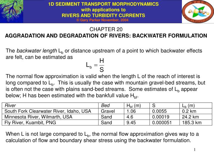
CHAPTER 20 AGGRADATION AND DEGRADATION OF RIVERS: BACKWATER FORMULATION The backwater length Lb or distance upstream of a point to which backwater effects are felt, can be estimated as The normal flow approximation is valid when the length L of the reach of interest is long compared to Lb. This is usually the case with mountain gravel-bed streams, but is often not the case with plains sand-bed streams. Some estimates of Lb appear below; H has been estimated with the bankfull value Hbf. When L is not large compared to Lb, the normal flow approximation gives way to a calculation of flow and boundary shear stress using the backwater formulation.
KEY FEATURES OF THE BACKWATER FORMULATION Just as in the normal flow formulation, water discharge per unit width qw is conserved, and is given by the relation and shear stress is related to flow velocity using a Chezy or Manning-Strickler formulation; Shear stress is no longer calculated from the depth-slope product, but instead from the full backwater equation; or thus
DOWNSTREAM BOUNDARY CONDITION FOR THE BACKWATER FORMULATION Base level is specified in terms of a prescribed downstream water surface elevation d(t) = (L, t) +H(L, t) rather than downstream bed elevation (L, t). The base level of the Athabasca River, Canada is controlled by the water surface elevation of Lake Athabasca. Delta of the Athabasca River at Lake Athabasca, Canada. Image from NASA https://zulu.ssc.nasa.gov/mrsid/mrsid.pl
THE MORPHODYNAMIC PROBLEM The formulation below uses a Manning-Strickler resistance formulation as an example. Exner equation Bed material load equation Backwater equation Specified initial bed Specified bed material feed rate Downstream boundary condition, or base level set in terms of specified water surface elevation.
CHARACTER OF THE MORPHODYNAMIC PROBLEM The normal flow assumption leads to a nonlinear diffusion problem. The backwater assumption leads to a nonlinear advection-diffusion problem. The difference between the two formulations is best shown, however in terms of linearized versions of the equations. In the analysis below Cf is taken to be constant for simplicity. To this end we consider perturbations about the mobile-bed equilibrium base state of Chapter 13, with depth Ho, bed slope So flow velocity Uo and bed material load qto, where The actual flow has depth H, slope S and bed material load qt which, differ from the base state, and evolves toward it according to the morphodynamics of the problem. The following non-dimensionalizations are introduced;
DIMENSIONLESS FORMULATION The morphodynamic problem takes the dimensionless form where denote values of the Shields and Froude numbers of the base flow.
PERTURBATION ABOUT THE BASE STATE Consider a case for which the deviatoric bed slope is small, i.e. and for which and deviate only slightly from unity. Setting where the following expressions are obtained upon Taylor expansion; where Nh is an order-one constant (except right near the threshold of motion).
REDUCTION TO LINEARIZED MORPHODYNAMIC PROBLEM and yield yields into Substituting or solving for , Substituting into yields
DIFFUSION AND ADVECTION The linearized form of the morphodynamic problem is thus: The first two terms are what results if backwater effects are ignored; they describe the following diffusion equation. The extra term on the right adds an advective component. To see this, consider for simplicity the balance associated with the two terms on the right-hand side of the equation;
ILLUSTRATION OF ADVECTION The equation has solutions of the form , where f is an arbitrary function and denotes a dimensionless wave velocity. That is, so that the top equation reduces to The neglected term in the full morphodynamic equation (top of previous slide) acts to damp these migrating waveforms. They propagate downstream for subcritical flow (Fro < 1) and upstream for supercritical flow (Fro > 1).
NUMERICAL SOLUTION TO THE BACKWATER FORMULATION OF MORPHODYNAMICS The case of subcritical flow is considered here. At any given time t the bed profile (x, t) is known. Solve the backwater equation upstream from x = L over this bed subject to the boundary condition Evaluate the Shields number and the bed material transport rate from the relations Find the new bed at time t + t Repeat using the bed at t + t
Honey, could you scratch my back, it itches in a place I can’t reach. IN MORPHODYNAMICS THE FLOW AND THE BED TALK TO AND INTERACT WITH EACH OTHER Sure, sweetie, but could you cut my toenails for me afterward? I can’t reach ‘em very well either.
THE PROBLEM OF IMPULSIVELY RAISED WATER SURFACE ELEVATION (BASE LEVEL) AT t = 0 M1 backwater curve qta qta Note: the M1 backwater curve was introduced in Chapter 5.
RESPONSE TO IMPULSIVELY RAISED WATER SURFACE ELEVATION: A PROGRADING DELTA THAT FILLS THE SPACE CREATED BY BACKWATER See Hotchkiss and Parker (1991) for more details.
NUMERICAL MODEL: INITIAL AND BOUNDARY CONDITIONS The channel is assumed to have uniform grain size D and some constant ambient slope S (before changing conditions at t = 0) which is in equilibrium with an ambient upstream feed rate qtf. The initial bed profile is thus the same as the one used for the calculations using the normal flow approximation; where for example Id can be set equal to zero. The boundary condition at the upstream end is also the same as before; where qtf(t) is a specified function. The downstream boundary condition, however, differs from that used in the normal flow calculation, and takes the form where d(t) is a specified function. Note that as opposed to the normal flow calculation, downstream bed elevation (L,t) is no longer specified, and is free to vary during the run.
NUMERICAL MODEL: DISCRETIZATION AND BACKWATER CURVE The discretization is the same as that used for the normal flow calculation. The backwater calculation over a given bed proceeds as in Chapter 5: where i proceeds downward from M to 1.
NUMERICAL MODEL: SEDIMENT TRANSPORT AND EXNER With a backwater formulation problem is not purely diffusional and a value of au greater than 0.5 (upwinding) may be necessary for numerical stability. The difference qt,1 is computed using the sediment feed rate at the ghost node:
INTRODUCTION TORTe-bookAgDegBW.xls The basic program in Visual Basic for Applications is contained in Module 1, and is run from worksheet “Calculator”. The program is designed to compute a) an ambient mobile-bed equilibrium, and the response of a reach to either b) changed sediment input rate at the upstream end of the reach starting from t = 0 or c) changed downstream water surface elevation at the downstream end of the reach starting from t = 0. The first set of required input includes: flood discharge Q, intermittency If, channel (bankfull) width B, grain size D, bed porosity p, composite roughness height kc and ambient bed slope S (before increase in sediment supply). Composite roughness height kc should be equal to ks = nkD, where nk is in the range 2 – 4, in the absence of bedforms. When bedforms are expected kc should be estimated at bankfull flow using the techniques of Chapter 9 and 10 (compute Cz from hydraulic resistance formulation, kc = (11 H)/exp(Cz)). Various parameters of the ambient flow, including the ambient annual bed material transport rate Gt in tons per year, are then computed directly on worksheet “Calculator”.
INTRODUCTION TORTe-bookAgDegBW.xls contd. The next required input is the annual average bed material feed rate Gtf imposed after t > 0. If this is the same as the ambient rate Gt (and downstream water surface elevation is not changed from the ambient value da) then nothing should happen; if Gtf > Gt then the bed should aggrade, and if Gtf < Gt then it should degrade. The next required input is the imposed downstream water surface elevation d. If this value equals the ambient value da (and the sediment feed rate is not altered from the ambient value Gt) then nothing should happen; if d > da then the bed should aggrade, and if d < da the bed should degrade. The imposed value d should not be so low as to force the flow to become supercritical; the worksheet provides guidance in this regard. The final set of input includes the reach length L, the number of intervals M into which the reach is divided (so that x = L/M), the time step t, the upwinding coefficient au, and two parameters controlling output, the number of time steps to printout Ntoprint and the number of printouts (in addition to the initial ambient state) Nprint. A value of au > 0.5 is recommended for stability.
INTRODUCTION TORTe-bookAgDegBW.xls contd. Auxiliary parameters, including r (coefficient in Manning-Strickler), t and nt (coefficient and exponent in load relation), c* (critical Shields stress), s (fraction of boundary shear stress that is skin friction) and R (sediment submerged specific gravity) are specified in the worksheet “Auxiliary Parameters”. The parameter s estimating the fraction of boundary shear stress that is skin friction, should either be set equal to 1 or estimated using the techniques of Chapter 9. In any given case it will be necessary to play with the parameters M (which sets x) and t in order to obtain good results. For any given x, it is appropriate to find the largest value of t that does not lead to numerical instability. The program is executed by clicking the button “Do a Calculation” from the worksheet “Calculator”. Output for bed elevation is given in terms of numbers in worksheet “ResultsofCalc” and in terms of plots in worksheet “PlottheData” The formulation is given in more detail in the worksheet “Formulation”.
MODULE 1 Sub Do_Fluvial_Backwater Sub Do_Fluvial_Backwater() Dim Hpred As Double: Dim fr2p As Double: Dim fr2 As Double: Dim fnp As Double: Dim fn As Double: Dim Cf As Double Dim i As Integer H(M + 1) = xio - eta(M + 1) For i = 1 To M fr2p = qw ^ 2 / g / H(M + 2 - i) ^ 3 Cf = (1 / alr ^ 2) * (H(M + 2 - i) / kc) ^ (-1 / 3) fnp = (eta(M + 1 - i) - eta(M + 2 - i) - Cf * fr2p * dx) / (1 - fr2p) Hpred = H(M + 2 - i) - fnp fr2 = qw ^ 2 / g / Hpred ^ 3 fn = (eta(M + 1 - i) - eta(M + 2 - i) - Cf * fr2 * dx) / (1 - fr2) H(M + 1 - i) = H(M + 2 - i) - 0.5 * (fnp + fn) Next i For i = 1 To M xi(i) = eta(i) + H(i) Next i End Sub
MODULE 1 Sub Find_Shields_Stress_and_Load Sub Find_Shields_Stress_and_Load() Dim i As Integer Dim taux As Double: Dim qstarx As Double: Dim Cfx As Double For i = 1 To M + 1 Cfx = (1 / alr ^ 2) * (H(i) / kc) ^ (-1 / 3) taux = Cfx * (qw / H(i)) ^ 2 / (Rr * g * D) If taux > tausc Then qstarx = alt * (fis * taux - tausc) ^ nt Else qstarx = 0 End If qt(i) = ((Rr * g * D) ^ 0.5) * D * qstarx Next i End Sub
A SAMPLE COMPUTATION Downstream water surface elevation is increased from 4.456 m (ambient value) to 15 m at t = 0 without altering the sediment feed rate.
RESULTS OF CALCULATION: A PROGRADING DELTA!!
PROGRADING DELTA ASSOCIATED WITH AN M1 BACKWATER CURVE The deep, slow-flowing M1 backwater zone created by ponding of water creates accomodation space in which sediment can be stored. As sediment progrades into the ponded zone, the leading edge of progradation sharpens into a migrating delta. A delta is an elevation shock, or zone over which elevation changes (reduces in this case) rapidly. The formulation of RTe-bookAgDegBW.xls is “shock-capturing;” that is, the numerical method automatically captures the delta. In such a formulation, the foreset slope of the delta is determined by the density of the numerical grid rather than physical parameters. A “shock-fitting” technique that allows the prescription of the foreset slope is given in Chapter 34. In the next slide the value of Ntoprint is varied to show the delta at various times.
DEGRADATION DRIVEN BY AN M2 BACKWATER CURVE The formulation can also handle degradation driven by an M2 backwater curve (Chapter 5). This is created when the downstream water surface elevation is lowered below the value associated with normal flow. An example is shown in the next slide. The input is the same as that of Slide 23 except that a) the imposed downstream water surface elevation is set at 2.25 m, i.e. below the ambient normal value of 4.456 m (so forcing an M2 backwater curve) and b) Ntoprint is varied to show the degradation at various times. If the downstream water surface elevation is set to a value that is so low that the outflow is Froude-supercritical the calculation will fail. Worksheet “Calculator” of RTe-bookAgDegBW.xls provides guidance in this regard (see rows 31-35). It is by no means impossible to treat the case of supercritical outflow. In general, however, such a treatment requires the abandonment of the quasi-steady approximation of Chapter 13.
REFERENCES FOR CHAPTER 20 Hotchkiss, R. H. and Parker, G., 1991, Shock fitting of aggradational profiles due to backwater, Journal of Hydraulic Engineering, 117(9): 1129‑1144. .