Download
1 / 33
360 likes | 538 Views
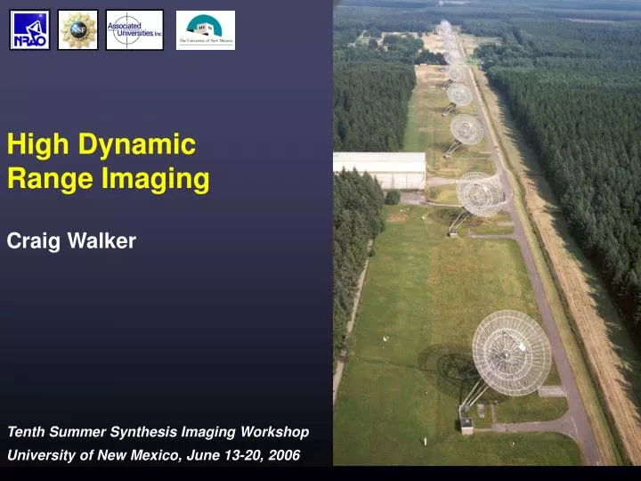
High Dynamic Range Imaging. Craig Walker. WHAT IS HIGH DYNAMIC RANGE IMAGING? AND WHY DO IT?. Accurate imaging with a high brightness ratio. High quality imaging of strong sources Flux evolution of components Motions of components Detection of weak features

E N D
High Dynamic Range Imaging Craig Walker
WHAT IS HIGH DYNAMIC RANGE IMAGING?AND WHY DO IT? • Accurate imaging with a high brightness ratio. • High quality imaging of strong sources • Flux evolution of components • Motions of components • Detection of weak features • Imaging of weak sources near strong sources • Deal with strongest sources in deep surveys • Deal with confusing sources near specific targets • Note some spectacular images have low dynamic range • Cygnus A, Cas A Tenth Summer Synthesis Imaging Workshop, UNM, June 13-20, 2006
QUALITY MEASURES • Dynamic range: • Usually is ratio of peak to off-source rms • Easy to measure • A measure of the ability to detect weak features • Highest I am aware of as of 2004: ~500,000 on 3C84 with WSRT • Fidelity: • Error of on-source features • Important for motion measurements, flux histories etc. • Hard to measure – don't know the "true" source • Mainly good for simulations • On-source errors typically much higher than off-source rms • Highest dynamic ranges are achieved on simple sources Tenth Summer Synthesis Imaging Workshop, UNM, June 13-20, 2006
WSRT 3C84 IMAGE J. Noordam, LOFAR calibration memo. Tenth Summer Synthesis Imaging Workshop, UNM, June 13-20, 2006
EXAMPLE: 3C120 VLA 6cm Image properties: Peak 3.12 Jy. Off-source rms 12 μJy/beam. Dynamic Range 260000. Knot at 4" is about 20 mJy/beam = 1/160 times core flux. Science question 1: Is the 4" knot superluminal? Rate near core is 0.007 times VLA beam per year. Answer after 13 years – subluminal. Science question 2: Chandra sees X-rays in circled region. What is the radio flux density? Needed to try to deduce emission mechanism. Radio is seen, barely, in this image. Tenth Summer Synthesis Imaging Workshop, UNM, June 13-20, 2006
EXAMPLE: SKA SURVEY Simulation from Windhorst et al. SKA memo which references Hopkins et al. Survey 1 square degree to 20 nJy rms in 12 hr with 0.1" beam • Required dynamic range 107 • There will typically be a ~200 mJy source in the field • Any long integration will have to deal with this problem • Dense UV coverage required • About 10 sources per sq. deg. above 100 nJy. • Significant fraction of sky filled • The EVLA will face the same issues, although to a lesser degree HST field size (<<1deg) Tenth Summer Synthesis Imaging Workshop, UNM, June 13-20, 2006
BASIC REQUIREMENTS FOR HIGH DYNAMIC RANGE IMAGING • A way to view the problem: It must be possible to subtract the model from the data with high accuracy • The model must be a good description of the sky • Typically clean components or MEM image • Need very good calibration and edit • Deal with commonly ignored effects • Closure errors • Spurious correlation, RFI etc. • Finite bandwidth and sources with spatial variations in spectral index • Position dependent gains due to primary beam shape and pointing • Position dependent gains due to troposphere and ionosphere • 3D effects for wide fields • Avoid digital precision effects (mostly a future issue) Tenth Summer Synthesis Imaging Workshop, UNM, June 13-20, 2006
UV COVERAGE • Obtain adequate UV coverage to constrain source • If divide UV plane into cells of about 1/(source size), need more sampled cells than there are beam areas covering the source • In other words, you need more constraints than unknowns • As dynamic range increases, beam areas with emission usually does too. • Avoid hidden distributions • Big UV holes • Missing short spacings • Can do simple sources with poor UV coverage • Example - 3C84 on the VLBA is a marginal case Tenth Summer Synthesis Imaging Workshop, UNM, June 13-20, 2006
EDITING CONSIDERATIONS • A few individual bad points don't have much effect • For typical data, phase errors are more important than amplitude errors • Example: a 5° phase error is equivalent to a 9% amplitude error • Small systematic errors can have a big cumulative effect • Nearly all editing should be station based • Most data problems are due to a problem at an antenna • Most clipping algorithms don't do this, which is a problem • Exceptions often relate to spurious correlation • RFI, DC offsets, pulse cal tones …. Tenth Summer Synthesis Imaging Workshop, UNM, June 13-20, 2006
SELF-CALIBRATION • High dynamic range imaging requires self-calibration • Atmosphere limits dynamic range to about 1000 for nodding calibration • High dynamic range is possible with just self-calibration • Nodding calibration is not required – get more time on-source • Typical VLBI case, but also true on VLA – see 3C120 example • But absolute position is not constrained – will match input model • Many iterations may be needed • Most true for complex sources and/or poor UV coverage • May need to vary parameters to help convergence • Robustness, UV range, taper, solution interval etc. Tenth Summer Synthesis Imaging Workshop, UNM, June 13-20, 2006
CLOSURE ERRORS • The measured visibility V'ijfor true visibility Vijis: V'ij = gi(t) g*j(t) Gij(t) Vij(t) + εij(t)+ єij(t) From the self-calibration chapter • gi(t) is a complex antenna gain • Initially measured on calibrators • Improved with self-calibration • Depends on sky position for large fields (comparable to primary beam) • Gij(t) is the portion of the gain that cannot be factored by antenna • These are the closure errors • The harmful variety are usually slowly or not variable • εij(t) is an additive offset term • For example spurious correlation of RFI etc. • These are also closure errors – the gain cannot be factored by antenna • Usually ignored • єij(t) is the thermal noise Tenth Summer Synthesis Imaging Workshop, UNM, June 13-20, 2006
CLOSURE ERRORS:EXTREME MISMATCHED BANDPASS EXAMPLE The average amplitudes on each baseline cannot be described in terms of antenna dependent gains Tenth Summer Synthesis Imaging Workshop, UNM, June 13-20, 2006
CLOSURE ERRORS: WHY THEY MATTER • Closure errors (Gij(t)) are typically small • VLA continuum: of order 0.5% • VLBA and VLA line: less than 0.1% • Often smaller than data noise • But the harmful closure errors are systematic • All data points on a given baseline may have the same offset • Small systematic errors mount up • Any data error is reduced in the image by about 1/N where N is the number of independent values • For noise, each data point is independent and N is the number of visibilities, which is large • For many closure errors, N is only the number of baselines • Nbas Nant Tenth Summer Synthesis Imaging Workshop, UNM, June 13-20, 2006
AVOIDING CLOSURE ERRORS (1) • Use accurate delays and/or narrow frequency channels • A delay error causes a phase slope with frequency • Averaging can cause baseline dependent smearing - does not close • Instrumental delays need to be removed accurately • VLA continuum system needs accurately set delays on-line • Delay changes with sky position, so wide fields need narrow channels • Use sufficiently short time averages to avoid smearing • Such smearing is baseline dependent - does not close • Troposphere, Ionosphere, Poor geometric model • Offset positions in wide field imaging • Well matched bandpasses • Mismatched bandpasses cause closure errors • Use bandpass calibration to reduce effect Tenth Summer Synthesis Imaging Workshop, UNM, June 13-20, 2006
AVOIDING CLOSURE ERRORS (2) • Avoid spurious correlations at low total fringe rate • Signals that can correlate: RFI, clipper offsets, pulse cal tones • VLA uses orthogonal Walsh functions to prevent correlation of clipper offsets. EVLA will use small frequency offsets • Happens on short baselines, polar sources and near V=0 • Can even be a problem for VLBI • Quantization correction (Van Vleck correction) • At high correlation, ratio of true/measured correlation is non-linear • This is a digital correlator effect for samples with few bits. • A concern when flux density >10% of SEFD • Avoid or calibrate the effect of polarization impurity on the parallel hand data • May be current VLA limiting factor Tenth Summer Synthesis Imaging Workshop, UNM, June 13-20, 2006
AVOIDING CLOSURE ERRORS (3) • Avoid or calibrate instrumental errors • Example: Non-orthogonality of real and imaginary signals from Hilbert transformer in VLA continuum causes closure errors. • Raw phase dependent • Limits VLA continuum system dynamic range to about 20,000 • Can hold constant by using array phasing • Calibrate on strong source • Avoid poor coherence - causes closure errors • Keep calibration solution intervals short compared to coherence time Tenth Summer Synthesis Imaging Workshop, UNM, June 13-20, 2006
CALIBRATING CLOSURE ERRORS • Avoid closure errors if possible by using appropriate observation parameters • Baseline calibration on strong calibrator • After best self cal, assume time averaged residual on each baseline is a closure error • Need high SNR • Errors in the calibrator model can transfer to data • Most problematic for polar sources and snaphot calibrator observations • Closure self-calibration • A baseline calibration on the target source • Depends on closure offsets being constant while UV structure is not • Will perfectly reproduce the model for snapshot • Some risk of matching the model even with long observations Tenth Summer Synthesis Imaging Workshop, UNM, June 13-20, 2006
IMAGING ISSUES FOR HIGH DYNAMIC RANGE • Digital representation: • For CLEAN, negative components are required to represent an unresolved feature between cells • Don't stop CLEAN or self-cal at first negative • If possible, put bright points on grid cells • Need 5 or 6 cells per beam • 32 bit real numbers may not be adequate for SKA • Use the most appropriate deconvolution algorithm • MEM for large, smooth sources • CLEAN for compact sources • NNLS best for partially resolved sources (avoid Briggs effect) • Don't use CLEAN boxes that are too large • CLEAN can fit the noise with a few points and give spurious low rms Tenth Summer Synthesis Imaging Workshop, UNM, June 13-20, 2006
LARGE FIELD IMAGING ISSUES • Position dependent gain: • Primary beam • Scales with frequency • Varies with pointing • Squint: RCP & LCP beams offset for asymmetric antennas (VLA, VLBA) • Rotates with hour angle • Isoplanatic patch – ionosphere or troposphere variations in position • Bandwidth and time average smearing away from center • May need to deal with confusing sources • Can be outside primary beam main lobe – separate self-cal • Bigger problem as sensitivity increases (serious for SKA) • Serious problem at low frequencies • Topic of active research in algorithms Tenth Summer Synthesis Imaging Workshop, UNM, June 13-20, 2006
LIMITS IMPOSED BY VARIOUS ERRORS Numbers are approximate maximum dynamic range • Atmosphere without self-calibration: 1,000 • Closure errors VLA continuum: 20,000 • Closure errors VLA line or VLBA: >100,000 • Uncalibrated closure errors (after baseline calibration) • VLA: >200,000 • WSRT: >400,000 • Thermal noise + maximum source strength > 106 • Very few sources are bright enough to reach this limit with current instruments. • Bigger problem with EVLA and especially SKA Tenth Summer Synthesis Imaging Workshop, UNM, June 13-20, 2006
EXAMPLE: 3C273 VLA 2nd self-cal (amp and phase) No self-cal 1st phase self-cal B Array Rotated so jet is vertical From R. Perley Synthesis Imaging Chapter 13. Tenth Summer Synthesis Imaging Workshop, UNM, June 13-20, 2006
3C273 RESIDUAL DATA Data - Model Points above 1 Jy from correlator malfunction. Points below 1 Jy mostly show closure errors 1 Jy UV Distance Tenth Summer Synthesis Imaging Workshop, UNM, June 13-20, 2006
EXAMPLE: 3C273 CONTINUED Bad baseline removed Self-closure calibration Clip residuals Tenth Summer Synthesis Imaging Workshop, UNM, June 13-20, 2006
EXAMPLE: VALUE OF SHORT BASELINES VLA A only VLA A+B Tenth Summer Synthesis Imaging Workshop, UNM, June 13-20, 2006
WIDE FIELD EXAMPLE • Sources in cluster Abell 2192 • Continuum from HI line cube (z=0.2) • Provided by Marc Verheijen • Bright source in first primary beam sidelobe • 39 mJy after primary beam attenuation • Self-cal on the confusing source • Subtract from UV data • Self-cal on primary beam sources Tenth Summer Synthesis Imaging Workshop, UNM, June 13-20, 2006
WIDE FIELD EXAMPLE: EXTERNAL CALIBRATION ONLY Confusing source outside primary beam near bottom Tenth Summer Synthesis Imaging Workshop, UNM, June 13-20, 2006
WIDE FIELD EXAMPLE: SAMPLE PRIMARY BEAMS Beams from different antennas Note variations far from center Tenth Summer Synthesis Imaging Workshop, UNM, June 13-20, 2006
WIDE FIELD EXAMPLE: SELF-CAL ON CONFUSING SOURCE Tenth Summer Synthesis Imaging Workshop, UNM, June 13-20, 2006
WIDE FIELD EXAMPLE:FINAL IMAGE Confusing source subtracted Self-cal on primary beam sources Tenth Summer Synthesis Imaging Workshop, UNM, June 13-20, 2006
Dan Briggs at the 1998 school, shortly before his death while skydiving BRIGGS EFFECT The Briggs effect is a deconvolution problem with partially resolved sources • Interpolation between longest baselines poor • Not seen on unresolved sources • Not seen on well resolved sources • Seen with all common deconvolution algorithms (CLEAN, MEM …) • Dan developed the NNLS algorithm which works • Non-Negative Least Squares • Restricted to sources of modest size (computer limitations) Tenth Summer Synthesis Imaging Workshop, UNM, June 13-20, 2006
BRIGGS EFFECT EXAMPLE: 3C48 UV DATA Tenth Summer Synthesis Imaging Workshop, UNM, June 13-20, 2006
BRIGGS EFFECT EXAMPLE: 3C48 IMAGES Tenth Summer Synthesis Imaging Workshop, UNM, June 13-20, 2006
THE END Tenth Summer Synthesis Imaging Workshop, UNM, June 13-20, 2006