Download
1 / 86
910 likes | 2.13k Views
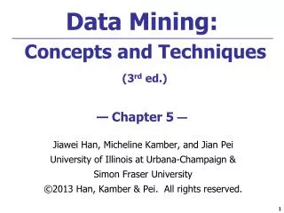
Data Mining: Concepts and Techniques (3 rd ed.) — Chapter 5 —. Jiawei Han, Micheline Kamber, and Jian Pei University of Illinois at Urbana-Champaign & Simon Fraser University ©2013 Han, Kamber & Pei. All rights reserved. 1. Chapter 5: Data Cube Technology.

E N D
Data Mining: Concepts and Techniques(3rd ed.)— Chapter 5 — Jiawei Han, Micheline Kamber, and Jian Pei University of Illinois at Urbana-Champaign & Simon Fraser University ©2013 Han, Kamber & Pei. All rights reserved. 1
Chapter 5: Data Cube Technology Data Cube Computation: Preliminary Concepts Data Cube Computation Methods Processing Advanced Queries by Exploring Data Cube Technology Multidimensional Data Analysis in Cube Space Summary 3
all 0-D(apex) cuboid time item location supplier 1-D cuboids time,item time,location item,location location,supplier 2-D cuboids time,supplier item,supplier time,location,supplier time,item,location 3-D cuboids item,location,supplier time,item,supplier 4-D(base) cuboid time, item, location, supplierc Data Cube: A Lattice of Cuboids 4
0-D(apex) cuboid time item location supplier 1-D cuboids time,item time,location item,location location,supplier 2-D cuboids item,supplier time,supplier time,location,supplier 3-D cuboids time,item,location item,location,supplier time,item,supplier 4-D(base) cuboid time, item, location, supplier Data Cube: A Lattice of Cuboids all • Base vs. aggregate cells; ancestor vs. descendant cells; parent vs. child cells • (9/15, milk, Urbana, Dairy_land) • (9/15, milk, Urbana, *) • (*, milk, Urbana, *) • (*, milk, Urbana, *) • (*, milk, Chicago, *) • (*, milk, *, *)
Cube Materialization: Full Cube vs. Iceberg Cube Full cube vs. iceberg cube compute cube sales iceberg as select month, city, customer group, count(*) from salesInfo cube by month, city, customer group having count(*) >= min support iceberg condition • Computing only the cuboid cells whose measure satisfies the iceberg condition • Only a small portion of cells may be “above the water’’ in a sparse cube • Avoid explosive growth: A cube with 100 dimensions • 2 base cells: (a1, a2, …., a100), (b1, b2, …, b100) • How many aggregate cells if “having count >= 1”? • What about “having count >= 2”? 6
Iceberg Cube, Closed Cube & Cube Shell • Is iceberg cube good enough? • 2 base cells: {(a1, a2, a3 . . . , a100):10, (a1, a2, b3, . . . , b100):10} • How many cells will the iceberg cube have if having count(*) >= 10? Hint: A huge but tricky number! • Close cube: • Closed cell c: if there exists no cell d, s.t. d is a descendant of c, and d has the same measure value as c. • Closed cube: a cube consisting of only closed cells • What is the closed cube of the above base cuboid? Hint: only 3 cells • Cube Shell • Precompute only the cuboids involving a small # of dimensions, e.g., 3 • More dimension combinations will need to be computed on the fly For (A1, A2, … A10), how many combinations to compute?
Roadmap for Efficient Computation • General cube computation heuristics (Agarwal et al.’96) • Computing full/iceberg cubes: 3 methodologies • Bottom-Up: Multi-Way array aggregation (Zhao, Deshpande & Naughton, SIGMOD’97) • Top-down: • BUC (Beyer & Ramarkrishnan, SIGMOD’99) • H-cubing technique (Han, Pei, Dong & Wang: SIGMOD’01) • Integrating Top-Down and Bottom-Up: • Star-cubing algorithm (Xin, Han, Li & Wah: VLDB’03) • High-dimensional OLAP: A Minimal Cubing Approach (Li, et al. VLDB’04) • Computing alternative kinds of cubes: • Partial cube, closed cube, approximate cube, etc. 8
General Heuristics (Agarwal et al. VLDB’96) • Sorting, hashing, and grouping operations are applied to the dimension attributes in order to reorder and cluster related tuples • Aggregates may be computed from previously computed aggregates, rather than from the base fact table • Smallest-child: computing a cuboid from the smallest, previously computed cuboid • Cache-results: caching results of a cuboid from which other cuboids are computed to reduce disk I/Os • Amortize-scans: computing as many as possible cuboids at the same time to amortize disk reads • Share-sorts: sharing sorting costs cross multiple cuboids when sort-based method is used • Share-partitions: sharing the partitioning cost across multiple cuboids when hash-based algorithms are used 9
Chapter 5: Data Cube Technology Data Cube Computation: Preliminary Concepts Data Cube Computation Methods Multi-Way Array Aggregation BUC High-Dimensional OLAP Processing Advanced Queries by Exploring Data Cube Technology Multidimensional Data Analysis in Cube Space Summary 10
Multi-Way Array Aggregation • Array-based “bottom-up” algorithm • Using multi-dimensional chunks • No direct tuple comparisons • Simultaneous aggregation on multiple dimensions • Intermediate aggregate values are re-used for computing ancestor cuboids • Cannot do Apriori pruning: No iceberg optimization 11
C c3 61 62 63 64 c2 45 46 47 48 c1 29 30 31 32 c 0 B 60 13 14 15 16 b3 44 28 56 9 b2 B 40 24 52 5 b1 36 20 1 2 3 4 b0 a0 a1 a2 a3 A Multi-way Array Aggregation for Cube Computation (MOLAP) • Partition arrays into chunks (a small subcube which fits in memory). • Compressed sparse array addressing: (chunk_id, offset) • Compute aggregates in “multiway” by visiting cube cells in the order which minimizes the # of times to visit each cell, and reduces memory access and storage cost. What is the best traversing order to do multi-way aggregation? 12
The best order is the one that minimizes the memory requirement and reduced I/Os Multi-way Array Aggregation for Cube Computation (3-D to 2-D)
Multi-way Array Aggregation for Cube Computation (2-D to 1-D)
Multi-Way Array Aggregation for Cube Computation (Method Summary) • Method: the planes should be sorted and computed according to their size in ascending order • Idea: keep the smallest plane in the main memory, fetch and compute only one chunk at a time for the largest plane • Limitation of the method: computing well only for a small number of dimensions • If there are a large number of dimensions, “top-down” computation and iceberg cube computation methods can be explored 15
Bottom-Up Computation (BUC) • BUC (Beyer & Ramakrishnan, SIGMOD’99) • Bottom-up cube computation (Note: top-down in our view!) • Divides dimensions into partitions and facilitates iceberg pruning • If a partition does not satisfy min_sup, its descendants can be pruned • If minsup = 1 Þ compute full CUBE! • No simultaneous aggregation 16
BUC: Partitioning • Usually, entire data set can’t fit in main memory • Sort distinct values • partition into blocks that fit • Continue processing • Optimizations • Partitioning • External Sorting, Hashing, Counting Sort • Ordering dimensions to encourage pruning • Cardinality, Skew, Correlation • Collapsing duplicates • Can’t do holistic aggregates anymore! 17
High-Dimensional OLAP? — The Curse of Dimensionality • None of the previous cubing method can handle high dimensionality! • A database of 600k tuples. Each dimension has cardinality of 100 and zipf of 2. 18
Motivation of High-D OLAP • X. Li, J. Han, and H. Gonzalez, High-Dimensional OLAP: A Minimal Cubing Approach, VLDB'04 • Challenge to current cubing methods: • The “curse of dimensionality’’ problem • Iceberg cube and compressed cubes: only delay the inevitable explosion • Full materialization: still significant overhead in accessing results on disk • High-D OLAP is needed in applications • Science and engineering analysis • Bio-data analysis: thousands of genes • Statistical surveys: hundreds of variables 19
Fast High-D OLAP with Minimal Cubing • Observation: OLAP occurs only on a small subset of dimensions at a time • Semi-Online Computational Model • Partition the set of dimensions into shell fragments • Compute data cubes for each shell fragment while retaining inverted indices or value-list indices • Given the pre-computed fragment cubes, dynamically compute cube cells of the high-dimensional data cube online 20
Properties of Proposed Method • Partitions the data vertically • Reduces high-dimensional cube into a set of lower dimensional cubes • Online re-construction of original high-dimensional space • Lossless reduction • Offers tradeoffs between the amount of pre-processing and the speed of online computation 21
Example: Computing a 5-D Cube with Two Shell Fragments • Let the cube aggregation function be count • Divide the 5-D table into 2 shell fragments: (A, B, C) and (D, E) • Build traditional invert index or RID list 22
Generalize the 1-D inverted indices to multi-dimensional ones in the data cube sense Compute all cuboids for data cubes ABC and DE while retaining the inverted indices For example, shell fragment cube ABC contains 7 cuboids: A, B, C AB, AC, BC ABC This completes the offline computation stage Cell Intersection TID List List Size a1 b1 1 2 3 1 4 5 1 1 a1 b2 1 2 3 2 3 2 3 2 a2 b1 4 5 1 4 5 4 5 2 a2 b2 4 5 2 3 0 Shell Fragment Cubes: Ideas 23
Shell Fragment Cubes: Size and Design • Given a database of T tuples, D dimensions, and F shell fragment size, the fragment cubes’ space requirement is: • For F < 5, the growth is sub-linear • Shell fragments do not have to be disjoint • Fragment groupings can be arbitrary to allow for maximum online performance • Known common combinations (e.g.,<city, state>) should be grouped together. • Shell fragment sizes can be adjusted for optimal balance between offline and online computation 24
ID_Measure Table • If measures other than count are present, store in ID_measure table separate from the shell fragments 25
The Frag-Shells Algorithm • Partition set of dimension (A1,…,An) into a set of k fragments (P1,…,Pk). • Scan base table once and do the following • insert <tid, measure> into ID_measure table. • for each attribute value ai of each dimension Ai • build inverted index entry <ai, tidlist> • For each fragment partition Pi • build local fragment cube Si by intersecting tid-lists in bottom- up fashion. 26
Frag-Shells Dimensions D Cuboid EF Cuboid DE Cuboid ABC Cube DEF Cube 27
Online Query Computation: Query • A query has the general form • Each ai has 3 possible values • Instantiated value • Aggregate * function • Inquire ? function • For example, returns a 2-D data cube. 28
Online Query Computation: Method • Given the fragment cubes, process a query as follows • Divide the query into fragment, same as the shell • Fetch the corresponding TID list for each fragment from the fragment cube • Intersect the TID lists from each fragment to construct instantiated base table • Compute the data cube using the base table with any cubing algorithm 29
Online Query Computation: Sketch Instantiated Base Table Online Cube 30
Experiment: Size vs. Dimensionality (50 and 100 cardinality) • (50-C): 106 tuples, 0 skew, 50 cardinality, fragment size 3. • (100-C): 106 tuples, 2 skew, 100 cardinality, fragment size 2. 31
Experiments on Real World Data • UCI Forest CoverType data set • 54 dimensions, 581K tuples • Shell fragments of size 2 took 33 seconds and 325MB to compute • 3-D subquery with 1 instantiate D: 85ms~1.4 sec. • Longitudinal Study of Vocational Rehab. Data • 24 dimensions, 8818 tuples • Shell fragments of size 3 took 0.9 seconds and 60MB to compute • 5-D query with 0 instantiated D: 227ms~2.6 sec. 32
Chapter 5: Data Cube Technology Data Cube Computation: Preliminary Concepts Data Cube Computation Methods Processing Advanced Queries by Exploring Data Cube Technology Sampling Cube: X. Li, J. Han, Z. Yin, J.-G. Lee, Y. Sun, “Sampling Cube: A Framework for Statistical OLAP over Sampling Data”, SIGMOD’08 Multidimensional Data Analysis in Cube Space Summary 33
Statistical Surveys and OLAP • Statistical survey: A popular tool to collect information about a population based on a sample • Ex.: TV ratings, US Census, election polls • A common tool in politics, health, market research, science, and many more • An efficient way of collecting information (Data collection is expensive) • Many statistical tools available, to determine validity • Confidence intervals • Hypothesis tests • OLAP (multidimensional analysis) on survey data • highly desirable but can it be done well? 34
Surveys: Sample vs. Whole Population Data is only a sample of population 35
Problems for Drilling in Sampling Cube • OLAP on Survey (i.e., Sampling) Data • Semantics of query is unchanged, but input data is changed Data is only a sample of population but samples could be small when drilling to certain multidimensional space 36
Challenges for OLAP on Sampling Data Q: What is the average income of 19-year-old high-school students? A: Returns not only query result but also confidence interval • Computing confidence intervals in OLAP context • No data? • Not exactly. No data in subspaces in cube • Sparse data • Causes include sampling bias and query selection bias • Curse of dimensionality • Survey data can be high dimensional • Over 600 dimensions in real world example • Impossible to fully materialize 37
Confidence Interval • Confidence interval at : • x is a sample of data set; is the mean of sample • tc is the critical t-value, calculated by a look-up • is the estimated standard error of the mean • Example: $50,000 ± $3,000 with 95% confidence • Treat points in cube cell as samples • Compute confidence interval as traditional sample set • Return answer in the form of confidence interval • Indicates quality of query answer • User selects desired confidence interval 38
Efficient Computing Confidence Interval Measures • Efficient computation in all cells in data cube • Both mean and confidence interval are algebraic • Why confidence interval measure is algebraic? is algebraic where both s and l (count) are algebraic • Thus one can calculate cells efficiently at more general cuboids without having to start at the base cuboid each time 39
Boosting Confidence by Query Expansion • From the example: The queried cell “19-year-old college students” contains only 2 samples • Confidence interval is large (i.e., low confidence). why? • Small sample size • High standard deviation with samples • Small sample sizes can occur at relatively low dimensional selections • Collect more data?― expensive! • Use data in other cells? Maybe, but have to be careful 40
Query Expansion: Intra-Cuboid Expansion Intra-Cuboid Expansion • Combine other cells’ data into own to “boost” confidence • If share semantic and cube similarity • Use only if necessary • Bigger sample size will decrease confidence interval • Cell segment similarity • Some dimensions are clear: Age • Some are fuzzy: Occupation • May need domain knowledge • Cell value similarity • How to determine if two cells’ samples come from the same population? • Two-sample t-test (confidence-based) 41
Intra-Cuboid Expansion What is the average income of 19-year-old college students? Expand query to include 18 and 20 year olds? Vs. expand query to include high-school and graduate students? 42
Query Expansion: Inter-Cuboid Expansion • If a query dimension is • Not correlated with cube value • But is causing small sample size by drilling down too much • Remove dimension (i.e., generalize to *) and move to a more general cuboid • Can use two-sample t-test to determine similarity between two cells across cuboids • Can also use a different method to be shown later 43
Chapter 5: Data Cube Technology Data Cube Computation: Preliminary Concepts Data Cube Computation Methods Processing Advanced Queries by Exploring Data Cube Technology Multidimensional Data Analysis in Cube Space Summary 44
Data Mining in Cube Space • Data cube greatly increases the analysis bandwidth • Four ways to interact OLAP-styled analysis and data mining • Using cube space to define data space for mining • Using OLAP queries to generate features and targets for mining, e.g., multi-feature cube • Using data-mining models as building blocks in a multi-step mining process, e.g., prediction cube • Using data-cube computation techniques to speed up repeated model construction • Cube-space data mining may require building a model for each candidate data space • Sharing computation across model-construction for different candidates may lead to efficient mining
Complex Aggregation at Multiple Granularities: Multi-Feature Cubes Multi-feature cubes (Ross, et al. 1998): Compute complex queries involving multiple dependent aggregates at multiple granularities Ex. Grouping by all subsets of {item, region, month}, find the maximum price in 2010 for each group, and the total sales among all maximum price tuples select item, region, month, max(price), sum(R.sales) from purchases where year = 2010 cube by item, region, month: R such that R.price = max(price) Continuing the last example, among the max price tuples, find the min and max shelf live, and find the fraction of the total sales due to tuple that have min shelf life within the set of all max price tuples 46
Discovery-Driven Exploration of Data Cubes Hypothesis-driven exploration by user, huge search space Discovery-driven (Sarawagi, et al.’98) Effective navigation of large OLAP data cubes pre-compute measures indicating exceptions, guide user in the data analysis, at all levels of aggregation Exception: significantly different from the value anticipated, based on a statistical model Visual cues such as background color are used to reflect the degree of exception of each cell 47
Kinds of Exceptions and their Computation Parameters SelfExp: surprise of cell relative to other cells at same level of aggregation InExp: surprise beneath the cell PathExp: surprise beneath cell for each drill-down path Computation of exception indicator (modeling fitting and computing SelfExp, InExp, and PathExp values) can be overlapped with cube construction Exception themselves can be stored, indexed and retrieved like precomputed aggregates 48
Chapter 5: Data Cube Technology Data Cube Computation: Preliminary Concepts Data Cube Computation Methods Processing Advanced Queries by Exploring Data Cube Technology Multidimensional Data Analysis in Cube Space Summary 50