Download
1 / 59
630 likes | 1.32k Views
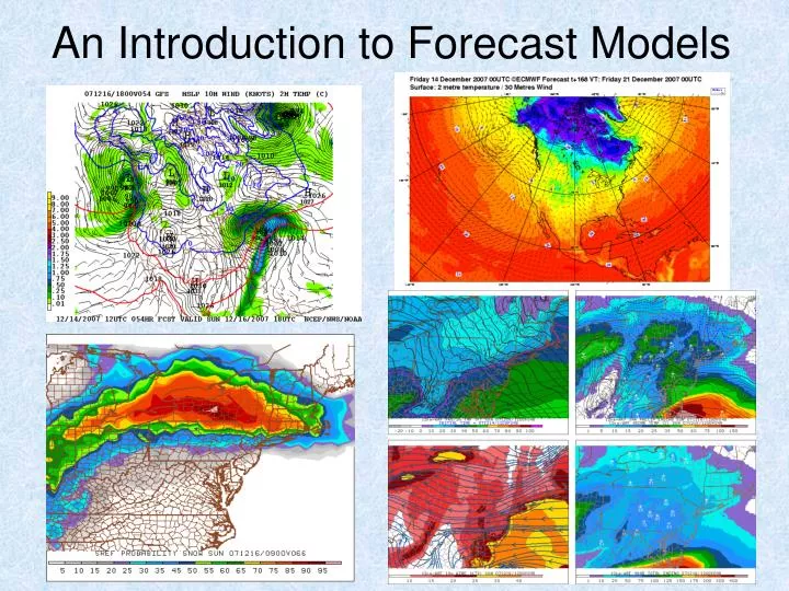
An Introduction to Forecast Models Outline Important Considerations: Atmospheric Science, Physical Processes. Weather Forecasting and Creating a Forecast Model. Model Construction and Resolution. Initialization and Model Run. Verification. Basics to Model Viewing, Time and Types of Data.

E N D
Outline • Important Considerations: Atmospheric Science, Physical Processes. • Weather Forecasting and Creating a Forecast Model. • Model Construction and Resolution. • Initialization and Model Run. • Verification. • Basics to Model Viewing, Time and Types of Data. • Model Types: Operational, Model Output Statistics, Ensembles. • Forecast Ranges: Short-Range, Medium-Range, Long-Range. • Model Access (sources of data). http://geocities.com/quincyq03/0207PPT.ppt
Why are models important to weather forecasting? • Weather is governed by laws of physics that are present in space, our atmosphere and at the Earth’s surface. • Equations have been derived and theorized to explain weather. • These equations are often very complex and the linear aspect does not sufficiently describe our atmosphere. • Calculus/differential equations are necessary for calculations. • These calculations take far too long to solve by hand and there are many variables that must be considered. • Forecast models have helped drastically improve forecasting skill, accuracy and verification.
Atmospheric Science • The study of Meteorology and forecasting is complex. • There are many processes taking place, in addition to many variables that affect weather patterns and events. • Global circulation causes radiative forcings, that due to the earth’s shape, creates wind and thermal gradients. • Daytime and nighttime due to sunrise and sunset also affect diurnal variances in wind and temperatures. • The shape of the earth’s orbit around the sun also creates seasons and variability in weather conditions, since there are times when parts of the earth’s surface are closer or farther away from the sun.
Atmospheric Science • Solar heating and radiation from the earth also take place. • Uneven surface heating due to many factors, including terrain and bodies of water, creates a further imbalance. • Drag and turbulence also play a role in the imbalance. • Storm systems and air masses are advected (transported) but are constantly evolving as well. • Storm systems spin up, develop, mature and weaken, while air masses are constantly modifying and moving. • Convergence and divergence of storm systems and air masses takes place…there is a LOT going on!
Processes and Variables to Consider • Even the previous slides only begin to graze the surface, as there is much more that drives weather! • Introductory Meteorology courses aim to introduce the student to just some of the basic fundamentals of Meteorology! Further courses, especially Dynamics and Thermodynamics get into more detailed and mathematical analyses of these processes. • The previous processes and variables all have calculated and/or theoretical equations to describe them. • Assumptions are made and without absolute knowledge, the equations are often approximate. • With that said, scientists have come to fairly accurate equations and methods of forecasting.
(From Holton’s An Introduction to Dynamic Meteorology) This image will be referred to again later in the presentation.
Weather Forecasting • Weather forecasting, up into the early 20th century, was largely very poor and often controversial. • Early forecasts were done by hand and were often fairly inaccurate, even within the short-range. • Some forecasts, such as short-term ones of pressure and temperature were decent, but scientists were beginning to realize that weather forecasting would improve with time, research and technological advances. • Weather prediction, through numerical calculation would be that next step. …Numerical Weather Prediction…
Creating a Forecast Model • Numerical Weather Prediction (NWP) was first proposed by Lewis Fry Richardson in 1920. "Richardson's Forecast Factory" Richardson knew that the amount of data that would need to be processed would be enormous, to create forecasts with accuracy and practical value. Today, computers are used to handle all of the information needed.
Creating a Forecast Model Networks of upper-air observation were introduced in the 1940s, allowing for tracking atmospheric data. Equations of atmospheric motion were studied and simplified, and by 1950, the first NWP experiments began. The first forecast computer model was created and it used the Barotropic Equation of Atmospheric motion to create 500hPa height forecasts. (hPa = millibar(mb)) Those forecasts out to 24 hours were significantly more accurate than any previous forecasts, but aside from the scientists, were not very practical or easy to understand.
Creating a Forecast Model • Further atmospheric equations were simplified and entered into forecast models. (numerous complex equations) • Computer technology evolved and allowed for more complex and accurate equations to be used over time. • As further research was done in the 1960s and 1970s, physicists and meteorologists were able to create more realistic, detailed and useful model forecasts. • With time, computer models have become and are becoming more able to process enormous amounts of data, which are necessary to create accurate forecasts.
Model Construction • The atmosphere is three-dimensional, the Earth is spherical and the surface is uneven. • Significant amounts of data must be input into forecast models to account for the variables to be considered. • Weather balloons are used for upper-air observation and information from many vertical levels are derived. • These observations are taken across the world at 12-hour intervals and cover both land and bodies of water.
Model Construction • Other data is also obtained from satellites, radar, ground/soil observations, the oceans and elsewhere. • Supercomputers are used to take all of this information in and from equations and theories, compute forecasts.
Model Construction (continued) • Think of a rectangular chunk of the world. • There is are east-west and north-south directions, but also an upward direction of altitude. • Computer models need three-dimensional coverage, so data at points across the earth surface (n, s, e, w) are input, but information is also added for specific heights above the ground.
Model Construction (continued) • Grid Points are equally spaced • locations that used to forecast the • weather through models. • Each grid point represents the average value for the air (volume) surrounding it, which can be considered an air parcel. • The grid points make up cubes that cover the earth’s surface, as well as extensions upward into the atmosphere to be 3-dimensional. • Atmospheric variables are represented through these grid points and since there is a finite number of them, finite difference approximations must be used to calculate variances.
Model Construction (continued) • A grid cell is the 3-dimensional cube that the grid cells combine to create. • The greater the number of grid points in a model, the smaller the grid cells become. • Smaller grid cells leads to greater model resolution and more detailed forecasts.
G R I D C E L L S
Model Resolution • The resolution of a model, is determined by the distance that separates the grid points. • For example, if the distance between two grid points on a model is 15km, the model resolution is 15km. • With research and technological capabilities, model resolution continues to improve. • The Nested Grid Model (NGM) has not been updated recently and is one of the lower resolution models today. • Mesoscale models, such as the MM5 and WRF/NAM have some of the highest resolutions.
Model Resolution • Model resolution does not necessarily mean more accurate forecasts… • In some ways, the lower resolution models give the best representation of the general weather patterns. • For more detailed forecasts, however, the lower resolution models tend to miss out on details, especially in the boundary layer (lower levels and surface). • All models have their uses and it depends on the forecaster viewing them and the particular weather event or pattern to determine which are best to use.
Model Initialization • The models take in observations, and through finite difference approximations, create a model initialization. • This initialization is a 00hr “forecast” that represents the current data that the model run will forecast from. • Depending on the model resolution and other parameters, that will determine what the 00hr data looks like. • Initializations tend to be similar between models at a given time, with only minor variations. • However, as will become more evident in subsequent discussions, sometimes bad data or poor initializations can lead to lower quality forecasts from that model run.
Example HPC Model Discussion MODEL DIAGNOSTIC DISCUSSION NWS HYDROMETEOROLOGICAL PREDICTION CENTER CAMP SPRINGS MD 1230 PM EST MON FEB 04 2008 VALID FEB 04/1200 UTC THRU FEB 08/0000 UTC MODEL INITIALIZATION... ...SEE NOUS42 KWNO ADMNFD FOR STATUS OF UPPER AIR INGEST... MODEL INITIALIZATION ERRORS DO NOT APPEAR TO HAVE A SIGNIFICANT IMPACT ON THE FCST. ...TROF PUSHING INTO THE W D1-2 AND THRU THE CNTRL CONUS D3... THE NAM IS TOO COLD WITH H85 TEMPS OVER WRN TX AND THE ADJACENT RIO GRANDE VLY BY UP TO 6 C. THE GFS HAD SIMILAR ISSUES...BUT NOT TO THE DEGREE OF THE NAM...WITH TEMPS OFF BY APPROX 2-3 C IN THE SAME LCNS. THE NAM AND GFS MAY BE TOO COLD WITH THE H85 TEMPS AHEAD OF THE TROF OVER THE SRN PLAINS/LWR MS VLY INTO THE FORECAST PD AS A RESULT. TO THE N...THE NAM...AND TO A LESSER EXTENT THE GFS...DID NOT DO A GOOD JOB INITIALIZING THE STRENGTH OF THE H85 TEMP GRADIENT OVER NERN CAN/ERN AK...WITH THE NAM AND GFS UP TO 3-4 C TOO WARM WITH THE COLD POOL OVER THE YUKON AND UP TO 4 C TOO COLD OVER NRN B.C./ALBERTA. SOME OF THIS AIRMASS IS XPCTD TO PHASE WITH THE TROF OVER CONUS LATER IN THE PD. THE NAM AND GFS MAY NOT BE ACCURATELY DEPICTING THESE AIRMASSES AND THE TEMP GRADIENT IN THE FORECAST PD.
Model Run • Once an initialization takes place, models then use the initialization data and equations to extrapolate a forecast. • Models need a method for time-stepping. (extrapolation) • Explicit Time Differencing involves the a predicted value to be determined at a given point for time step S+1, from the previous time step, S. • Implicit Time Differencing is more complicated and includes the steps of S+1 and S-1. • The latter system is more complicated and takes up much more computer power, but has many advantages.
Model Run • As a model continues a forecast from the starting time, 00(hr) and continue out from there. (+6hr, +12hr, etc) • Models are run out under their limitations and setups, until the process is adjusted or ends. • For example, with the Global Forecasting System (GFS), the model resolution is downscaled after 180 hours. • Model accuracy tends to decrease over time. • Since approximations are used at initialization and throughout the model run, such a decrease in accuracy with time can be expected. Also, the model is forecast potential scenarios, so that must be considered as well.
Model Run Delay • Models have so much data to ingest and work with, that there is typically a long delay for their forecasts. • Depending on the model, this delay may be anywhere from around 1 hour to even 6 or more hours! • For those of you who do view some model output, this explains why you have to wait a few hours after the initialization time to view the data!
Basics to Model Viewing • The time scale that the vast majority of the models use is Universal Time (UTC) • During Standard Time (fall/winter), UTC is 5 hours ahead of Eastern Standard Time. • During Daylight Savings Time, UTC is only 4 hours ahead of Eastern Savings Time. • UTC is also known as Zulu (z) time.
Main Types of Models • Operational models • The ones that are most common & numerous. • Model Output Statistics (MOS) • Adjusted operational model runs, based on statistics. • Ensembles • Several members with slight variations.
The Operational Model • This model is the standard run for most models. • The NWS Forecast Discussions will often refer to these runs as the “OP run”. • The GFS, NAM, ECMWF, GGEM, etc all have an operational model – the one used “the most”.
Model Output Statistics (MOS) • This model is based off of its operational counterpart, but has many adjustments to it. • MOS forecasts are used to fine-tune and adjust the operational output. • MOS will output more detailed information, than what can generally be derived from the OP run. • Statistical analyses are used to further adjust the forecasts for individual stations, seasons, etc.
More on MOS • The most common example of a MOS model would be the GFS MOS (MAV and MEX).
Ensemble Forecasts • Ensembles are created from the operational models in two different ways: • Different physical parameterizations • Various initial conditions. • Physical Parameterizations have to do with how models develop clouds, transfer energy, handle the boundary layer, etc. • Initial Conditions are the conditions that the models initialize from.
“The Two Ways” • Why different physical parameterizations? • Under some situations, the operational model may be more biased towards a certain, eventual outcome. • By viewing & comparing runs from different physical parameterizations, they can be analyzed better. • Why alter the initial conditions? • Consider a model run…the initialization is almost always off very slightly with all of the variables. • The model approximates initial conditions, so there is always some error across the board.
Physical Parameterizations • “The approximation of unresolved processes in terms of resolved variables is referred to as parameterization”.Holton 474 • Physical parameterizations in forecast models are very difficult, complex and aim to increase forecast accuracy. • The atmospheric (including boundary layer and surface) processes must be approximated and simulated. • Aside from Ensembles, other models also have various physical parameterization schemes. • This explains, in part, why some models seem to handle certain weather patterns or events differently.
Models have various schemes of evaluating and forecasting these processes.
Physical Parameterizations • The operational model run has set parameterizations, but each ensemble member may have slight variations. • The method of explaining/forecasting the processes is already approximate, so minor adjustments are added. • Each ensemble member will have slight variations, so as the model runs out, further forecast variations will arise. • Depending on the situation and the individual member, different scenarios will unfold. • Forecasters can compare and assess the ensemble members, to evaluate the operational run and also see what kind of spread and mean forecast is forecasted.
Altering Initial Conditions • The “Butterfly Effect” can be considered. • Instead of a butterfly slightly flapping its wings to throw off a forecast, slight deviations from the model initializations will cause a similar chain reaction. • This chain reaction explains why models are not perfect. • As a forecast model generates longer and longer forecasts, each proceeding interval has less and less accurate information to extrapolate from. • Although the initial conditions are important, there are often many minor errors in a given initialization.
Altering Initial Conditions • Ensemble models that use this method, take the “initial conditions” and adjust them slightly in several ways. • There are many ensemble members that now have slightly different initializations to work with. • The ensembles then extrapolate their forecasts and commonalities can be noticed – “Ensemble Mean”. • By viewing all of the different ensembles, we can evaluate the operational run and determine if the run looks accurate, or if it is more likely to be an outlier. • However, a difficulty with the ensembles is that sometimes the mean is far off from the actual verification and outliers may verify. Occasionally, the ensemble spread may not even cover the actual scenario!
Forecast Ranges • We will consider the short-range forecasts to include generally forecasts to go out to 72 hours or less. • The medium-range forecasts will be from 3 to 7 days. • Long-range forecasts include those beyond 7 days. • Different models have various forecast ranges.
Short-Range Forecasts • Short-range forecasts tend to focus on the exact details, such as temperature gradients, precipitation, and mesoscale phenomena. • These forecasts tend to originate from models with higher resolution. • When forecasting severe weather or precipitation types, these are useful for specifics. • However, a forecaster must also consider that models are not flawless and real-time data should also be considered.
Examples of SR Models • WRF/NAM: Forecasts out to 84 hours. • SREF: Short-Range Ensemble Forecasts! • RUC: Rapid updates for out to 12 hours. • NGM: Lower resolution, but out to 48 hours. • MAV MOS: 72 hour forecasts. • RGEM: Regional GEM out to 48 hours.