Download
1 / 71
730 likes | 895 Views
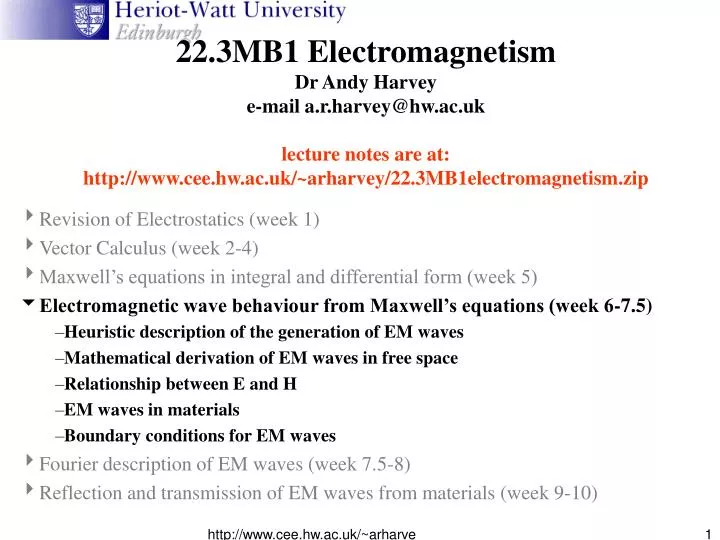
22.3MB1 Electromagnetism Dr Andy Harvey e-mail a.r.harvey@hw.ac.uk lecture notes are at: http://www.cee.hw.ac.uk/~arharvey/22.3MB1electromagnetism.zip. Revision of Electrostatics (week 1) Vector Calculus (week 2-4) Maxwell’s equations in integral and differential form (week 5)

E N D
22.3MB1 ElectromagnetismDr Andy Harveye-mail a.r.harvey@hw.ac.uklecture notes are at:http://www.cee.hw.ac.uk/~arharvey/22.3MB1electromagnetism.zip Revision of Electrostatics (week 1) Vector Calculus (week 2-4) Maxwell’s equations in integral and differential form (week 5) Electromagnetic wave behaviour from Maxwell’s equations (week 6-7.5) Heuristic description of the generation of EM waves Mathematical derivation of EM waves in free space Relationship between E and H EM waves in materials Boundary conditions for EM waves Fourier description of EM waves (week 7.5-8) Reflection and transmission of EM waves from materials (week 9-10) http://www.cee.hw.ac.uk/~arharvey/22.3MB1electromagnetism.zip Dr Andy Harvey
Maxwell’s equations in differential form • Varying E and H fields are coupled NB Equations brought from elsewhere, or to be carried on to next page, highlighted in this colour NB Important results highlighted in this colour http://www.cee.hw.ac.uk/~arharvey/22.3MB1electromagnetism.zip Dr Andy Harvey
Fields at large distances from charges and current sources • For a straight conductor the magnetic field is given by Ampere’s law • At large distances or high frequencies H(t,d) lags I(t,d=0) due to propagation time • Transmission of field is not instantaneous • Actually H(t,d) is due to I(t-d/c,d=0) • Modulation of I(t) produces a dH/dt term H I • dH/dt produces E • dE/dt term produces H • etc. • How do the mixed-up E and H fields spread out from a modulated current ? • eg current loop, antenna etc http://www.cee.hw.ac.uk/~arharvey/22.3MB1electromagnetism.zip Dr Andy Harvey
A moving point charge: • A static charge produces radial field lines • Constant velocity, acceleration and finite propagation speed distorts the field line • Propagation of kinks in E field lines which produces kinks of and • Changes in E couple into H & v.v • Fields due to are short range • Fields due to propagate • Accelerating charges produce travelling waves consisting coupled modulations of E and H http://www.cee.hw.ac.uk/~arharvey/22.3MB1electromagnetism.zip Dr Andy Harvey
E in plane of page H in and out of page Depiction of fields propagating from an accelerating point charge • Fields propagate at c=1/me=3 x 108 m/sec http://www.cee.hw.ac.uk/~arharvey/22.3MB1electromagnetism.zip Dr Andy Harvey
Examples of EM waves due to accelerating charges • Bremstrahlung - “breaking radiation” • Synchrotron emission • Magnetron • Modulated current in antennas • sinusoidal v.important • Blackbody radiation http://www.cee.hw.ac.uk/~arharvey/22.3MB1electromagnetism.zip Dr Andy Harvey
2.2 Electromagnetic waves in lossless media - Maxwell’s equations Constitutive relations Maxwell SI Units • J Amp/ metre2 • D Coulomb/metre2 • H Amps/metre • B Tesla Weber/metre2 Volt-Second/metre2 • E Volt/metre • e Farad/metre • m Henry/metre • s Siemen/metre Equation of continuity http://www.cee.hw.ac.uk/~arharvey/22.3MB1electromagnetism.zip Dr Andy Harvey
2.6 Wave equations in free space • In free space • s=0 J=0 • Hence: • Taking curl of both sides of latter equation: http://www.cee.hw.ac.uk/~arharvey/22.3MB1electromagnetism.zip Dr Andy Harvey
Wave equations in free space cont. • It has been shown (last week) that for any vector A where is the Laplacian operator Thus: • There are no free charges in free space so .E=r=0 and we get A three dimensional wave equation http://www.cee.hw.ac.uk/~arharvey/22.3MB1electromagnetism.zip Dr Andy Harvey
What does this mean • dimensional analysis ? • moe has units of velocity-2 • Why is this a wave with velocity 1/ moe ? Wave equations in free space cont. • Both E and H obey second order partial differential wave equations: http://www.cee.hw.ac.uk/~arharvey/22.3MB1electromagnetism.zip Dr Andy Harvey
v The wave equation • Why is this a travelling wave ? • A 1D travelling wave has a solution of the form: Substitute back into the above EM 3D wave equation Constant for a travelling wave This is a travelling wave if • In free space http://www.cee.hw.ac.uk/~arharvey/22.3MB1electromagnetism.zip Dr Andy Harvey
Wave equations in free space cont. • Substitute this 1D expression into 3D ‘wave equation’ (Ey=Ez=0): • Sinusoidal variation in E or H is a solution ton the wave equation http://www.cee.hw.ac.uk/~arharvey/22.3MB1electromagnetism.zip Dr Andy Harvey
Summary of wave equations in free space cont. • Maxwells equations lead to the three-dimensional wave equation to describe the propagation of E and H fields • Plane sinusoidal waves are a solution to the 3D wave equation • Wave equations are linear • All temporal field variations can be decomposed into Fourier components • wave equation describes the propagation of an arbitrary disturbance • All waves can be written as a superposition of plane waves (again by Fourier analysis) • wave equation describes the propagation of arbitrary wave fronts in free space. http://www.cee.hw.ac.uk/~arharvey/22.3MB1electromagnetism.zip Dr Andy Harvey
Summary of the generation of travelling waves • We see that travelling waves are set up when • accelerating charges • but there is also a field due to Coulomb’s law: • For a spherical travelling wave, the power carried by the travelling wave obeys an inverse square law (conservation of energy) • P a E2 a 1/r2 • to be discussed later in the course • Ea1/r • Coulomb field decays more rapidly than travelling field • At large distances the field due to the travelling wave is much larger than the ‘near-field’ http://www.cee.hw.ac.uk/~arharvey/22.3MB1electromagnetism.zip Dr Andy Harvey
due to charge constant velocity (1/ r2) due to E (1/r) Heuristic summary of the generation of travelling waves E due to stationary charge (1/r2) kinks due to charge acceleration (1/r) http://www.cee.hw.ac.uk/~arharvey/22.3MB1electromagnetism.zip Dr Andy Harvey
2.8 Uniform plane waves - transverse relation of E and H • Consider a uniform plane wave, propagating in the z direction. E is independent of x and y In a source free region, .D=r =0 (Gauss’ law) : E is independent of x and y, so • So for a plane wave, E has no component in the direction of propagation. Similarly for H. • Plane waves have only transverse E and H components. http://www.cee.hw.ac.uk/~arharvey/22.3MB1electromagnetism.zip Dr Andy Harvey
Orthogonal relationship between E and H: • For a plane z-directed wave there are no variations along x and y: • Equating terms: • and likewise for : • Spatial rate of change of H is proportionate to the temporal rate of change of the orthogonal component of E & v.v. at the same point in space http://www.cee.hw.ac.uk/~arharvey/22.3MB1electromagnetism.zip Dr Andy Harvey
Orthogonal and phase relationship between E and H: • Consider a linearly polarised wave that has a transverse component in (say) the y direction only: • Similarly • H and E are in phase and orthogonal http://www.cee.hw.ac.uk/~arharvey/22.3MB1electromagnetism.zip Dr Andy Harvey
Note: • The ratio of the magnetic to electric fields strengths is:which has units of impedance • and the impedance of free space is: http://www.cee.hw.ac.uk/~arharvey/22.3MB1electromagnetism.zip Dr Andy Harvey
Orientation of E and H • For any medium the intrinsic impedance is denoted by hand taking the scalar productso E and H are mutually orthogonal • Taking the cross product of E and H we get the direction of wave propagation http://www.cee.hw.ac.uk/~arharvey/22.3MB1electromagnetism.zip Dr Andy Harvey
A ‘horizontally’ polarised wave • Sinusoidal variation of E and H • E and H in phase and orthogonal Hy Ex http://www.cee.hw.ac.uk/~arharvey/22.3MB1electromagnetism.zip Dr Andy Harvey
A block of space containing an EM plane wave • Every point in 3D space is characterised by • Ex, Ey, Ez • Which determine • Hx, Hy, Hz • and vice versa • 3 degrees of freedom l Ex Hy http://www.cee.hw.ac.uk/~arharvey/22.3MB1electromagnetism.zip Dr Andy Harvey
An example application of Maxwell’s equations:The Magnetron http://www.cee.hw.ac.uk/~arharvey/22.3MB1electromagnetism.zip Dr Andy Harvey
The magnetron Lorentz force F=qvB • Locate features: Poynting vector S Displacement current, D Current, J http://www.cee.hw.ac.uk/~arharvey/22.3MB1electromagnetism.zip Dr Andy Harvey
Power flow of EM radiation • Intuitively power flows in the direction of propagation • in the direction of EH • What are the units of EH? • hH2=.(Amps/metre)2 =Watts/metre2 (cf I2R) • E2/h=(Volts/metre)2 /=Watts/metre2 (cf I2R) • Is this really power flow ? http://www.cee.hw.ac.uk/~arharvey/22.3MB1electromagnetism.zip Dr Andy Harvey
dx l Ex Hy Area A Power flow of EM radiation cont. • Energy stored in the EM field in the thin box is: • Power transmitted through the box is dU/dt=dU/(dx/c).... http://www.cee.hw.ac.uk/~arharvey/22.3MB1electromagnetism.zip Dr Andy Harvey
Power flow of EM radiation cont. • This is the instantaneous power flow • Half is contained in the electric component • Half is contained in the magnetic component • E varies sinusoidal, so the average value of S is obtained as: • S is the Poynting vector and indicates the direction and magnitude of power flow in the EM field. http://www.cee.hw.ac.uk/~arharvey/22.3MB1electromagnetism.zip Dr Andy Harvey
Example problem • The door of a microwave oven is left open • estimate the peak E and H strengths in the aperture of the door. • Which plane contains both E and H vectors ? • What parameters and equations are required? • Power-750 W • Area of aperture - 0.3 x 0.2 m • impedance of free space - 377 W • Poynting vector: http://www.cee.hw.ac.uk/~arharvey/22.3MB1electromagnetism.zip Dr Andy Harvey
Solution http://www.cee.hw.ac.uk/~arharvey/22.3MB1electromagnetism.zip Dr Andy Harvey
Suppose the microwave source is omnidirectional and displaced horizontally at a displacement of 100 km. Neglecting the effect of the ground: • Is the E-field a) vertical b) horizontal c) radially outwards d) radially inwards e) either a) or b) • Does the Poynting vector point a) radially outwards b) radially inwards c) at right angles to a vector from the observer to the source • To calculate the strength of the E-field should one a) Apply the inverse square law to the power generated b) Apply a 1/r law to the E field generated c) Employ Coulomb’s 1/r2 law http://www.cee.hw.ac.uk/~arharvey/22.3MB1electromagnetism.zip Dr Andy Harvey
Field due to a 1 kW omnidirectional generator (cont.) http://www.cee.hw.ac.uk/~arharvey/22.3MB1electromagnetism.zip Dr Andy Harvey
4.1 Polarisation • In treating Maxwells equations we referred to components of E and H along the x,y,z directions • Ex, Ey, EzandHx, Hy, Hz • For a plane (single frequency) EM wave • Ez=Hz =0 • the wave can be fully described by either itsE components or its H components • It is more usual to describe a wave in terms of its E components • It is more easily measured • A wave that has the E-vector in the x-directiononly is said to be polarised in the x direction • similarly for the y direction http://www.cee.hw.ac.uk/~arharvey/22.3MB1electromagnetism.zip Dr Andy Harvey
Polarisation cont.. • Normally the cardinal axes are Earth-referenced • Refer to horizontally or vertically polarised • The field oscillates in one plane only and is referred to as linear polarisation • Generated by simple antennas, some lasers, reflections off dielectrics • Polarised receivers must be correctly aligned to receive a specific polarisation A horizontal polarised wave generated by a horizontal dipole and incident upon horizontal and vertical dipoles http://www.cee.hw.ac.uk/~arharvey/22.3MB1electromagnetism.zip Dr Andy Harvey
Horizontal and vertical linear polarisation http://www.cee.hw.ac.uk/~arharvey/22.3MB1electromagnetism.zip Dr Andy Harvey
Linear polarisation • If both Ex and Ey are present and in phase then components add linearly to form a wave that is linearly polarised signal at angle f Horizontal polarisation Vertical polarisation Co-phased vertical+horizontal =slant Polarisation http://www.cee.hw.ac.uk/~arharvey/22.3MB1electromagnetism.zip Dr Andy Harvey
Slant linear polarisation Slant polarised waves generated by co-phased horizontal and vertical dipoles and incident upon horizontal and vertical dipoles http://www.cee.hw.ac.uk/~arharvey/22.3MB1electromagnetism.zip Dr Andy Harvey
Circular polarisation LHC polarisation NB viewed as approaching wave RHC polarisation http://www.cee.hw.ac.uk/~arharvey/22.3MB1electromagnetism.zip Dr Andy Harvey
Circular polarisation LHC RHC LHC & RHC polarised waves generated by quadrature -phased horizontal and vertical dipoles and incident upon horizontal and vertical dipoles http://www.cee.hw.ac.uk/~arharvey/22.3MB1electromagnetism.zip Dr Andy Harvey
Elliptical polarisation - an example http://www.cee.hw.ac.uk/~arharvey/22.3MB1electromagnetism.zip Dr Andy Harvey
Constitutive relations • permittivity of free space e0=8.85 x 10⁻¹² F/m • permeability of free space mo=4px10-7 H/m • Normally er(dielectric constant) andmr • vary with material • are frequency dependant • For non-magnetic materials mr ~1 and for Fe is ~200,000 • eris normally a few ~2.25 for glass at optical frequencies • are normally simple scalars (i.e. for isotropic materials) so that D and E are parallel and B and H are parallel • For ferroelectrics and ferromagnetics er andmr depend on the relative orientation of the material and the applied field: At microwave frequencies: http://www.cee.hw.ac.uk/~arharvey/22.3MB1electromagnetism.zip Dr Andy Harvey
Constitutive relations cont... • What is the relationship between e and refractive index for non magnetic materials ? • v=c/n is the speed of light in a material of refractive index n • For glass and many plastics at optical frequencies • n~1.5 • er~2.25 • Impedance is lower within a dielectric What happens at the boundary between materials of different n,mr,er ? http://www.cee.hw.ac.uk/~arharvey/22.3MB1electromagnetism.zip Dr Andy Harvey
Why are boundary conditions important ? • When a free-space electromagnetic wave is incident upon a medium secondary waves are • transmitted wave • reflected wave • The transmitted wave is due to the E and H fields at the boundary as seen from the incident side • The reflected wave is due to the E and H fields at the boundary as seen from the transmitted side • To calculate the transmitted and reflected fields we need to know the fields at the boundary • These are determined by the boundary conditions http://www.cee.hw.ac.uk/~arharvey/22.3MB1electromagnetism.zip Dr Andy Harvey
Boundary Conditions cont. m1,e1,s1 m2,e2,s2 • At a boundary between two media, mr,ers are different on either side. • An abrupt change in these values changes the characteristic impedance experienced by propagating waves • Discontinuities results in partial reflection and transmission of EM waves • The characteristics of the reflected and transmitted waves can be determined from a solution of Maxwells equations along the boundary http://www.cee.hw.ac.uk/~arharvey/22.3MB1electromagnetism.zip Dr Andy Harvey
m1,e1,s1 m2,e2,s2 E2t, H2t • The normal component of D is continuous at the surface of a discontinuity if there is no surface charge density. If there is surface charge density D is discontinuous by an amount equal to the surface charge density. • D1n,=D2n+rs • The normal component of B is continuous at the surface of discontinuity • B1n,=B2n D1n, B1n m1,e1,s1 m2,e2,s2 D2n, B2n 2.3 Boundary conditions E1t, H1t • The tangential component of E is continuous at a surface of discontinuity • E1t,=E2t • Except for a perfect conductor, the tangential component of H is continuous at a surface of discontinuity • H1t,=H2t http://www.cee.hw.ac.uk/~arharvey/22.3MB1electromagnetism.zip Dr Andy Harvey
m1,e1,s1 m2,e2,s2 0 0 0 0 0 Proof of boundary conditions - continuity of Et • Integral form of Faraday’s law: That is, the tangential component of E is continuous http://www.cee.hw.ac.uk/~arharvey/22.3MB1electromagnetism.zip Dr Andy Harvey
m1,e1,s1 m2,e2,s2 0 0 0 0 0 Proof of boundary conditions - continuity of Ht • Ampere’s law That is, the tangential component of H is continuous http://www.cee.hw.ac.uk/~arharvey/22.3MB1electromagnetism.zip Dr Andy Harvey
Proof of boundary conditions - Dn • The integral form of Gauss’ law for electrostatics is: m1,e1,s1 m2,e2,s2 applied to the box gives hence The change in the normal component of D at a boundary is equal to the surface charge density http://www.cee.hw.ac.uk/~arharvey/22.3MB1electromagnetism.zip Dr Andy Harvey
Proof of boundary conditions - Dn cont. • For an insulator with no static electric charge rs=0 • For a conductor all charge flows to the surface and for an infinite, plane surface is uniformly distributed with area charge densityrs In a good conductor, s is large, D=eE0 hence if medium 2 is a good conductor http://www.cee.hw.ac.uk/~arharvey/22.3MB1electromagnetism.zip Dr Andy Harvey
Proof of boundary conditions - Bn • Proof follows same argument as for Dn on page 47, • The integral form of Gauss’ law for magnetostatics is • there are no isolated magnetic poles The normal component of B at a boundary is always continuous at a boundary http://www.cee.hw.ac.uk/~arharvey/22.3MB1electromagnetism.zip Dr Andy Harvey
2.6 Conditions at a perfect conductor • In a perfect conductor s is infinite • Practical conductors (copper, aluminium silver) have very large s and field solutions assuming infinite s can be accurate enough for many applications • Finite values of conductivity are important in calculating Ohmic loss • For a conducting medium • J=sE • infinite s infinite J • More practically, s is very large, E is very small (0) and J is finite http://www.cee.hw.ac.uk/~arharvey/22.3MB1electromagnetism.zip Dr Andy Harvey