Download
1 / 35
350 likes | 555 Views
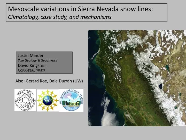
Mesoscale variations in Sierra Nevada snow lines: C limatology , case study, and mechanisms. Justin Minder Yale Geology & Geophysics David Kingsmill NOAA-ESRL (HMT). Also: Gerard Roe, Dale Durran (UW). Mountain snow and climate change.

E N D
Mesoscale variations in Sierra Nevada snow lines: Climatology, case study, and mechanisms Justin Minder Yale Geology & Geophysics David Kingsmill NOAA-ESRL (HMT) Also: Gerard Roe, Dale Durran(UW)
Mountain snow and climate change The partitioning between rain & snow has big impacts on both hydrological resources & hazards What role to mesoscale processes play in modulating the rain-snow transition over mountains?
wind Z0C δ0C δ δS z ZS x The mountainside snow line & mesoscale controls ZBB Z0C : Zero-degree line ZS: Snow line ZBB: Bright band elevation
Snowline observations: Case studies N. Sierra: Isotherms (oC) Altitude (km) Z0C Marwitz (1987) • Lowering of ZBB & Z0Cby up to 1km over: • N. Sierra Nevada • Oregon Cascades • Italian Alps Distance (km) Italian Alps: Reflectivity(dBZe) ZBB Medina et al. (2005)
Snowline observations: N. Sierra Climatology 2005/6 -2007/8 storm-based climatology ZBBdrops ZBBrises ~50km • Lowering of the snowline is a climatological feature • ΔZS ~100m’s, big enough for major impacts on snowpack and flooding What causes ΔZS(ΔZBB)and its variability?
Z 0C Z 0C Z S Why does the snowline dip downwards towards the terrain? Possible mechanisms Along-barrier transport of cool/dry air Pseudo-adiabatic cooling from lifting Z 0C Z 0C Cooling by melting of orographically enhanced snowfall Increased melting distance for orographically enhanced snowfall
2-D semi-idealized numerical simulations WRF-ARW (v3.0.1) Δx=2km 201 vertical eta-levels (Δz=20-400m) Open BCs in x Periodic BCs in y Free slip bottom boundary Thompson et al. bulk microphysics (6 phases, incl. Graupel) f-plane ( f = 10-4 s-1) w-damping Layer (Klemp 2009) RH = 20% Nd= 0.01 s-1 U stratosphere RH = 95% Nm = 0.005 s-1 U = 15 m s-1 hm ,a troposphere Initial conditions: Prescribe: Ts: temp. at z=0 Nm: moist stability RH : relative humidity U : cross-mountain winds Terrain: cos4 ridge, with prescribed: hm: height=1.5km a: half-width=40km Run to steady state
2D semi-idealized WRF simulations: Mechanisms wind Minder et al. (2011) ~45% ~30% ~20% Minder, JR, DR Durran, GH Roe, 2011: Mesoscale Controls on the Mountainside Snow-line. Journal of the Atmospheric Sciences, 68, 2107-2127.
2D semi-idealized WRF simulations: Sensitivity to Temperature Ts=3oC Ts=7oC • Z0C upwind rises 742 m with warming, ZS on the mountainside rises only 530 m. • Mesoscale processes “buffer” effects of warming on the snow-line by ~30%.
2D semi-idealized WRF simulations: Sensitivity to microphysics Minder et al. (2011) Microphysics
A case study of Northern Sierra Nevada snowline behavior Feb 8-12, 2007 • Do idealized results carry-over? • Do 3D dynamics, PBL fluxes, radiation, etc. change the answer? GOES IR (shading) & Sea Level pressure (contours)
Mesoscale Observations NOAA HMT-West profiler & balloons SHS BBD BLU CFC ATA profilers sfc. met. White et al. (2002) algorithm for ZBBdetection
Mesoscale Modeling • 72 hr simulation • Feb 8, 12 UTC – Feb 11, 12 UTC • 4 nested domains • (27km; 9km ; 3km; 1km) • IC’s and BC’s from NARR • Nudge doms. 1-2 towards NARR • 118 vertical levels • Δz = 30 m from 1-3km • Parameterizations: • WSM6 microphysics • Kain-Fritsch convection (d1-3) • MYJ boundarylayer OLR (shading) Sea Level Pressure (contours)
Surface (Precip. & Temp.) WRF Obs. Observations WRF T(°C) Precip (mm) Time (UTC; dd.hh) Time (UTC; dd.hh)
ZBB & Z0C : upwind vs. mountain Observations Z0C ZBB ΔBB= -110 m ΔBB= -140 m WRF Z0C ZBB ΔBB= -70m ΔBB= -210 m
WRF cross – section 1hr rainfall (shading) 500m winds (barbs) Frozen precip. mix. ratio (shading) y(km) Z0C wind x(km) ~20% • Full drop in Z0C& ZSis more like 400-600m (underestimated by profilers) • Causes? • ~100 m melting distance
Trajectory diagnostics (1): Pseudo-adiabatic mechanisms • Calculate 3-hr back-trajectories from model output, ending at Z0C on transect. Pseudo-adiabatic • Try to use simple pseudo-adiabatic parcel model to predict Z0C for each traj. • ~200 m pseudo-adiabatic (3D) “other” ~40% Total ΔZ0C
Trajectory diagnostics (2): Cooling by melting mechanism • Construct a θebudget for two representative trajectories 18 7 Δ • Δθe is almost entirely due to cooling by melting snow Total Cooling by melting Total Cooling by melting ~30% fhr fhr • ~150 m cooling from melting
Case study summary & further work • Still working on: • Sensitivity to microphysics • Sensitivity to temperature • Future plans: • Examine other cases (low snowline w/ more blocking) • More climatological analysis with HMT data • LES of melting layer turbulence • Examination of other settings ~20% ~30% ~40%
A mesoscale lowering of the snowline over terrain appears to be a common feature of mid-latitude mountain climate A range of pseudo-adiabatic, diabatic, & microphysical processes may explain this behavior These processes may be simulated and diagnosed in mesoscale numerical models, which suggest important roles for several mechanisms Conclusions The dependence of these mechanisms on climate may result in modulations of large-scale climate impacts Climate-connections are being further investigated using multi-year observations and regional climate models
Z0C ZS ZBB z z z Z0C Z0C Z0C Melting layer Bright band ZS ZBB T dbZ q s,g (q s,g)o/2 (q s,g)o 0ºC The atmospheric snowline The elevation in the atmosphere where falling snow melts into rain z zero-degree line bright-band height snow line
(δ)Dmelt What physical processes determine ZS?Role of: Melting Distance (Dmelt) (δ)Dmelt = (Z0C)mtn. - (ZS)mtn. (δ)Dmelt = 125 m qc (shading), Isotherms ( contours every 1oC)
(δ)Qmelt What physical processes determine ZS?Role of: Latent Cooling from Melting (Qmelt) ZS and Z0C from runs: with Qmelt (solid) without Qmelt (dashed) (δ)Qmelt = (δ0C) - (δ0C)no-Qmelt (δ)Qmelt = 61 m Advection through melting layer is too fast for substantial Qmelt qc (shading)
What physical processes determine ZS?Role of: pseudo-adiabatic Cooling (Qad.) Consider flow over a mountain that is: Steady Inviscid Stably stratified Pseudo-adiabatic Moist thermodynamics following air parcel determines δ0C Captured by simple air parcel model Γ Z Γm δ0C Z0C T(z) parcel environment dT/dz=Γ Ts Γd T 0°C Ts (δ0C)parcel depends on: Ts, Γ (Nm), RH (δ0C)parcel = 107 m c.f. WRF : (δ0C)no-Qmelt = 81 m (δ)Qad.= 81 m
What physical processes determine ZS?Summary (δ)Qad. Z0C δ (δ)Qmelt ZS z (δ)Dmelt x δ = (δ)Dmelt+ (δ)Qmelt+ (δ)Qad. 267m = 125 m + 61 m + 81 m …but how general is this result ?