Beyond Linear Separability

1. Beyond Linear Separability

2. Limitations of Perceptron • Only linear separations • Only converges for linearly separable data One Solution (SVM’s) Map data into a feature space where they are linearly separable Another solution is to use multiple interconnected perceptrons.

3. Artificial Neural Networks • Interconnected networks of simple units (let's call them "artificial neurons") in which each connection has a weight. • Weight wij is the weight of the ith input into unit j. • NN have some inputs where the feature values are placed and they compute one or more output values. • Depending on the output value we determine the class. • If there are more than one output units we choose the one with the greatest value. • The learning takes place by adjusting the weights in the network so that the desired output is produced whenever a sample in the input data set is presented.

4. Single Perceptron Unit • We start by looking at a simpler kind of "neural-like" unit called a perceptron. Depending on the value of h(x) it outputs one class or the other.

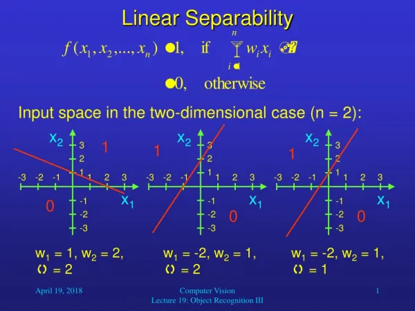
5. Beyond Linear Separability • Since a single perceptron unit can only define a single linear boundary, it is limited to solving linearly separable problems. • A problem like that illustrated by the values of the XOR boolean function cannot be solved by a single perceptron unit.

6. Multi-Layer Perceptron • Solution: Combine multiple linear separators. • The introduction of "hidden" units into NN make them much more powerful: • they are no longer limited to linearly separable problems. • Earlier layers transform the problem into more tractable problems for the latter layers.

7. Example: XOR problem Output: “class 0” or “class 1”

8. Example: XOR problem

9. Example: XOR problem w23o2+w13o1+w03=0 w03=-1/2, w13=-1, w23=1 o2-o1-1/2=0

10. Multi-Layer Perceptron • Any set of training points can be separated by a three-layer perceptron network. • “Almost any” set of points is separable by two-layer perceptron network.

11. Autonomous Land Vehicle In a Neural Network (ALVINN) • ALVINN is an automatic steering system for a car based on input from a camera mounted on the vehicle. • Successfully demonstrated in a cross-country trip.

12. ALVINN • The ALVINN neural network is shown here. It has • 960 inputs (a 30x32 array derived from the pixels of an image), • 4 hidden units and • 30 output units (each representing a steering command).

13. Optional material

14. Multi-Layer Perceptron Learning • However, the presence of the discontinuous threshold in the operation means that there is no simple local search for a good set of weights; • one is forced into trying possibilities in a combinatorial way. • The limitations of the single-layer perceptron and the lack of a good learning algorithm for multilayer perceptrons essentially killed the field for quite a few years.

15. Soft Threshold • A natural question to ask is whether we could use gradient ascent/descent to train a multi-layer perceptron. • The answer is that we can't as long as the output is discontinuous with respect to changes in the inputs and the weights. • In a perceptron unit it doesn't matter how far a point is from the decision boundary, we will still get a 0 or a 1. • We need a smooth output (as a function of changes in the network weights) if we're to do gradient descent.

16. Sigmoid Unit • The classic "soft threshold" that is used in neural nets is referred to as a "sigmoid" (meaning S-like) and is shown here. • The variable z is the "total input" or "activation" of a neuron, that is, the weighted sum of all of its inputs. • Note that when the input (z) is 0, the sigmoid's value is 1/2. • The sigmoid is applied to the weighted inputs (including the threshold value as before). • There are actually many different types of sigmoids that can be (and are) used in neural networks. • The sigmoid shown here is actually called the logistic function.

17. Training • The key property of the sigmoid is that it is differentiable. • This means that we can use gradient based methods of minimization for training. • The output of a multi-layer net of sigmoid units is a function of two vectors, the inputs (x) and the weights (w). • The output of this function (y) varies smoothly with changes in the input and, importantly, with changes in the weights.

18. Training

19. Training • Given a set of training points, each of which specifies the net inputs and the desired outputs, we can write an expression for the training error, usually defined as the sum of the squared differences between the actual output (given the weights) and the desired output. • The goal of training is to find a weight vector that minimizes the training error. • We could also use the mean squared error (MSE), which simply divides the sum of the squared errors by the number of training points instead of just 2. Since the number of training points is a constant, the value for which we get the minimum is not affected.

20. Training

21. Gradient Descent We've seen that the simplest method for minimizing a differentiable function is gradient descent (or ascent if we're maximizing). Recall that we are trying to find the weights that lead to a minimum value of training error. Here we see the gradient of the training error as a function of the weights. The descent rule is basically to change the weights by taking a small step (determined by the learning rate ) in the direction opposite this gradient. Online version: We consider each time only the error for one data item

22. Gradient Descent – Single Unit Substituting in the equation of previous slide we get (for the arbitrary ithelement): Delta rule

23. Derivative of the sigmoid

24. Generalized Delta Rule Now, let’s compute 4. z4 will influence E, only indirectly through z5 and z6.

26. Generalized Delta Rule In general, for a hidden unit j we have

27. Generalized Delta Rule For an output unit we have

28. Backpropagation Algorithm • Initialize weights to small random values • Choose a random sample training item, say (xm, ym) • Compute total input zj and output yj for each unit (forward prop) • Compute n for output layer n = yn(1-yn)(yn-ynm) • Compute j for all preceding layers by backprop rule • Compute weight change by descent rule (repeat for all weights) • Note that each expression involves data local to a particular unit, we don't have to look around summing things over the whole network. • It is for this reason, simplicity, locality and, therefore, efficiency that backpropagation has become the dominant paradigm for training neural nets.

29. Training Neural Nets • Now that we have looked at the basic mathematical techniques for minimizing the training error of a neural net, we should step back and look at the whole approach to training a neural net, keeping in mind the potential problem of overfitting. • Here we look at a methodology that attempts to minimize that danger.

30. Training Neural Nets Given: Data set, desired outputs and a neural net with m weights. Find a setting for the weights that will give good predictive performance on new data. • Split data set into three subsets: • Training set – used for adjusting weights • Validation set – used to stop training • Test set – used to evaluate performance • Pick random, small weights as initial values • Perform iterative minimization of error over training set (backprop) • Stop when error on validation set reaches a minimum (to avoid overfitting) • Repeat training (from step 2) several times (to avoid local minima) • Use best weights to compute error on test set.

31. y3 y1 y2 z3 z1 z2 Backpropagation Example First do forward propagation: Compute zi’s and yi’s. 3 w03 -1 w13 w23 1 2 w21 w12 w02 w01 w11 w22 -1 -1 x2 x1