Download
1 / 57
570 likes | 703 Views
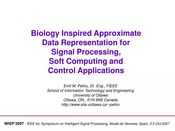
Biology Inspired Approximate Data Representation for Signal Processing, Soft Computing and Control Applications. Emil M. Petriu, Dr. Eng., FIEEE School of Information Technology and Engineering University of Ottawa Ottawa, ON., K1N 6N5 Canada http://www.site.uottawa.ca/~petriu.

E N D
Biology Inspired Approximate Data Representation for Signal Processing, Soft Computing and Control Applications Emil M. Petriu, Dr. Eng., FIEEE School of Information Technology and Engineering University of Ottawa Ottawa, ON., K1N 6N5 Canada http://www.site.uottawa.ca/~petriu WISP’2007 - IEEE Int. Symposium on Intelligent Signal Processing, Alcalá de Henares, Spain, 3-5 Oct.2007
Abstract This paper reviews basics, similarities, and applications of two biology inspired approximate data representation modalities: stochastic data representation and fuzzy linguistic variables.
Dendrites carry electrical signals in into the neuron body. The neuron body integrates and thresholds the incoming signals. The axon is a single long nerve fiber that carries the signal from the neuron body to other neurons. A synapse is the connection between dendrites of two neurons. Dendrites Body Synapse Axon Incoming signals to a dendrite may be inhibitory or excitatory. The strength of any input signal is determined by the strength of its synaptic connection. A neuron sends an impulse down its axon if excitation exceeds inhibition by a critical amount (threshold/ offset/bias) within a time window (period of latent summation). Memories are formed by the modification of the synaptic strengths which can change during the entire life of the neural systems. Biological neurons are rather slow (10-3 s) when compared with the modern electronic circuits. ==> The brain is faster than an electronic computer because of its massively parallel structure. The brain has approximately 1011 highly connected neurons (approx. 104 connections per neuron). Biological Neurons
Looking for a model to prove that algebraic operations with analog variables can be performed by logic gates, von Neuman advanced in 1956 the idea of representing analog variables by the mean rate of random-pulse streams [J. von Neuman, “Probabilistic logics and the synthesis of reliable organisms from unreliable components,” in Automata Studies, (C.E. Shannon, Ed.), Princeton, NJ, Princeton University Press, 1956].
The “random-pulse machine” concept, [S.T. Ribeiro, “Random-pulse machines,” IEEE Trans. Electron. Comp., vol. EC-16, no. 3, pp. 261-276,1967], a.k.a. "noise computer“, "stochastic computing“, “dithering” deals with analog variables represented by the mean rate of random-pulse streams allowing to use digital circuits to perform arithmetic operations. This concept presents a good tradeoff between the electronic circuit complexity and the computational accuracy. The resulting neural network architecture has a high packing density and is well suited for very large scale integration (VLSI).
Random-Pulse/Digital Conversion The deterministic component of the random-pulse sequence, conveniently unbiased and rescaled for this purpose to take values +1 and -1 (instead of 1 and respectively 0) , can be calculated as a statistical estimation from the quantization diagram: E[VRP] = (+1) .p[VR>=0] + (-1) .p[VR<0] = p(VRP) - p(VRP’) = (FS+V)/(2.FS) - (FS-V)/(2.FS )= V/FS; This finally gives the deterministic analog value V associated with the binary VRP sequence: V = [p(VRP) - p(VRP')] . FS ; where the apostrophe ( ' ) denotes a logical inversion.
- N N 1 1 1 å å = = + V * VRP ( VRP VRP ); N i i N N N = = i 1 i 1 - VRP VRP = + N 0 V * V * ; - N N 1 N Random-pulse/digital converter using the moving average algorithm .
Analog/random-pulse and random-pulse/digital conversion of a “step” input signal
S1 Sm Sj CLK x1 X1 1 OUT_OF m DEMULTIPLEXER y xj Xj Y = (X1+...+Xm)/m RANDOM NUMBER GENERATOR xm Xm Random-Pulse Addition
VRQ CLK CLOCK XQ D /2 D /2 VR + V X XQ b -BIT p.d.f. + D 1/ VRP QUANTIZER of VR R . . b D b D (1- ) k+1 ANALOG RANDOM p(R) SIGNAL . b D D 1/ GENERATOR R k 0 D D - /2 + /2 k-1 X . . 0 D ( k-0.5) D ( k+0.5) . b D V= (k- ) . D k Stochastic Data Representation Generalized b-bit analog/stochastic-data conversion and its quantization characteristics
The ideal estimation over an infinite number of samples of the stochastic data sequence VRD is: E[VRD] = (k-1). p[(k-1.5)D≤ VR < (k-0.5) D] + k . p[(k-0.5)D≤ VR< (k+0.5)D] = (k-1) . b + k . (1-b) = k -b The estimation accuracy of the recovered value for V depends on the quantization resolution, the finite number of samples that are actually averaged, and on the statistical properties of the analog dither.
Mean square errors function of the moving average window size
0 1 -1 Y 00 01 10 X 0 00 0 00 0 00 0 00 1 01 0 00 1 01 -1 10 -1 10 0 00 -1 10 1 01 Y X LSB LSB Z Y LSB LSB X Z MSB MSB 2-bit stochastic-data multiplier.
Correlator Architectures Using Stochastic Data Representation
- N 1 1 å · D = · D · - · D COR ( k t ) V 1 ( n t ) V 2 (( n k ) t ) V 1 V 2 N = n 0
- 1 N 1 å for k = 0,1,2,3. · D = · D · - · D COR ( k t ) x ( n t ) y (( n k ) t ) ; xy N = 0 n Parallel architecture of a 4-point correlator using random-pulse data representation.
Each calculated correlation point has a 8-bit resolution. In order to reduce the number of interface lines, the 8-bit wide outputs of the four random-pulse/digital converters are multiplexed. When more modules are connected in larger structures the 1-bit XRQ input lines of all modules are connected together while the 1-bit YRQ output of each module is connected to the 1-bit YRQ input of the next module creating a longer delay line.
Autocorrelation function of a sinusoid calculated by a 32-point parallel random-pulse correlator with a 8-bit/point resolution.
Correlation function of two sinusoids with the same frequency but different amplitudes and phases, calculated by a 32-point parallel random-pulse correlator with a 8-bit/point resolution.
Correlation function between a sinusoid and another sinusoid of the same frequency but corrupted by white noise, calculated by a32-point parallel random-pulse correlator with 8-bit/point resolution.
Neural Network Architectures Using Stochastic Data Representation
Multi-bit stochastic-data implementation of a synapse Multi-bit stochastic-data implementation of a neuron body.
a P n 30x1 W 30x1 30x1 30x30 P1, t1 P2, t2 P3, t3 30 Auto-associative memory NN architecture Recovery of 30% occluded patterns Training set
Fuzzy Logic Pioneered by Zadeh in the mid ‘60s fuzzy logic provides the formalism for modeling the approximate reasoning mechanisms specific to the human brain. “In more specific terms, what is central about fuzzy logic is that, unlike classical logical systems, it aims at modeling the imprecise modes of reasoning that play an essential role in the remarkable human ability to make rational decisions in an environment of uncertainty and imprecision. This ability depends, in turn, on our ability to infer an approximate answer to a question based on a store of knowledge that is inexact, incomplete, or not totally reliable.” [ “Fuzzy Logic,” IEEE Computer Magazine, April 1988, pp. 83-93: ]
Fuzzy Logic Control The basic idea of “fuzzy logic control” (FLC) was suggested by L.A. Zadeh, “A rationale for fuzzy control,” J. Dynamic Syst. Meas. Control, vol.94, series G, pp.3-4,1972. FLC provides a non analytic alternative to the classical analytic control theory. ==> “But what is striking is that its most important and visible application today is in a realm not anticipated when fuzzy logic was conceived, namely, the realm of fuzzy-logic-based process control,” [L.A. Zadeh, “Fuzzy logic,” IEEE Computer Mag., pp. 83-93, Apr. 1988]. Early FLCs were reported by Mamdani and Assilian in 1974, and Sugeno in 1985.
OUTPUT y* INPUT x* Classical control systems are based on a detailed I/O function OUTPUT= F (INPUT) mapping each high-resolution quantization interval of the input domain into a high-resolution quantization interval of the output domain
OUTPUT y* Defuzzification Fuzzification INPUT x* Fuzzy control is based on a much simpler functional description of the desired I/O behavior mapping each low-resolution quantization interval of the input domain into a low-resolution quantization interval of the output domain
Membership functions and the quantization characteristics for a 3-set (N, Z, and P) fuzzy partition of the domain where the analog variable x is defined. XFQare the crispanalog values recovered after a defuzzification of the fuzzy converted value x. It also shows the truncated information XQ recovered from an A/D converter with 3 quantization levels defined over the same domain for x.
The key benefit of FLC is that the desired system behavior can be described with simple “if-then” relations based on very low-resolution models able to incorporate empirical engineering knowledge. FLCs have found many practical applications in the context of complex ill-defined processes that can be controlled by skilled human operators: water quality control, automatic train operation control, elevator control, etc.,
b g q a d DOCK Fuzzy Controller for Truck and Trailer Docking
LH LM LS ZE RS RM RH NL NL NM NM NS NS ZE ZE PS PS PM PM PL PL STEER ( q ) AB (a-b) [deg.] -48 -38 -20 0 20 38 48 [deg.] -110-95 -35 -20 -10 0 10 20 35 95 110 SPEED GAMMA ( g ) [ % ] 16 24 30 [deg.] -85-55 -30 -15 -10 0 10 15 30 55 85 REV FWD DIRN NEAR FAR LIMIT DIST ( d ) [arbitrary] - + [m] 0.05 0.1 0.75 0.90 OUTPUT MEMBERSHIP FUNCTIONS INPUT MEMBERSHIP FUNCTIONS SLOW MED FAST
“STEER / DIRN” RULE BASE AB a-b ( ) GAMMA ( ) g NL NM NS ZE PS PM PL There is a hysteresis ring around the center of the rule base table for the DIRN output. This means that when the vehicle reaches a state within this ring, it will continue to drive in the same direction, F(forward) or R (reverse), as it did in the previous state outside this ring. A hysteresis was purposefully introduced to increase the robustness of the FLC. NL LH/F LH/F LM/F LS/F RS/F RM/F LH/F ZE RM LH LH LM NM RH/F LH/F F-R F-R F-R F-R F-R LH RM NS LH/F LM/R LS/R RS/R RH/F F-R F-R LH RH ZE LH/F LS/R ZE/R RS/R RH/F F-R F-R RH LM PS LH/F LS/R RS/R RM/R RH/F F-R F-R LM ZE RM RH RH RH/F PM LH/F F-R F-R F-R F-R F-R LS/F PL LM/F RS/F RM/F RH/F RH/F RH/F
q = (mLH. qLH +mLM. qLM + mLS. qLS + mZE. qZE + mRS. qRS +mRM. qRM + mRH. qRH ) / (mLH + mLM + mLS + mZE + mRS + mRM + mRL) q 63 63 g a-b 0 0 DEFFUZIFICATION The crisp value of the steering angle is obtained by the modified “centroidal” deffuzification (Mamdani inference): I/O characteristic of th Fuzzy Logic Controller for truck and trailer docking.
q q 16 16 g a-b 63 63 0 0 g a-b 0 0 STOCHASTIC-DATA FUZZY LOGIC CONTROLLERS There is tenet of common wisdom that FLCs are meant to successfully deal with uncertain data. According to this, FLCs are supposed to make do with “uncertain” data coming from (cheap) low-resolution and imprecise sensors. However, experiments show that the low resolution of the sensor data results in rough quantization of of the controller's I/O characteristic: 4-bit sensors 7-bit sensors I/O characteristics of the FLC for truck & trailer docking for 4-bit sensor data (a, b, g) and 7-bit sensor data.
Design a Fuzzy Logic Controller (FLC) able to back up a truck into a docking station from any initial position that has enough clearance from the docking station. The truck backing-up problem
The FLC is based on the Sugeno-style fuzzy inference. The fuzzy rule base consists of 35 rules.
Time diagram of digital FLC's output qduring a docking experiment when the input variables, j and x are analog and respectively quantizied with a 4-bit bit resolution
FLC architecture using 4-bit stochastic data representation with low-pass filters placed immediately after the input A/D converters
It offers a better performance • than the previous one because • a final low-pass filter can also • smooth the non-linearity caused • by the min-max composition • rules of the FLC. • FLC architecture using 4-bit stochastic data representation with low-pass filters placed at the FLC’s outputs.
Q [deg] 30 20 10 0 -10 -20 -30 -40 -50 0 10 20 30 40 50 60 70 Time (s) Time diagram of the stochastic FLC's output during a docking experiment when 4-bit A/D converters are used to quantize the dithered inputs and the low-pass filter is placed at the FLC's output