Download
1 / 49
500 likes | 599 Views
Standard Error and Research Methods. Claude Oscar Monet: Gare St. Lazare, 1877. The Goal of Sociology 302 In Sociology 302 we will learn how to collect data and measure concepts as accurately as possible.

E N D
Standard Error and Research Methods Claude Oscar Monet: Gare St. Lazare, 1877
The Goal of Sociology 302 In Sociology 302 we will learn how to collect data and measure concepts as accurately as possible. To understand why accuracy in data collection and concept measurement are important, we need to understand the statistical concept standard error and its use in science.
Standard Error Standard error is the extent to which an estimate, such as a mean of a distribution or the slope of a regression line, can vary, given a level of confidence (typically, 95% in sociological research). Standard error is the amount of “wiggle room” for our estimates: how much they can be larger or smaller than the true value of what we are attempting to estimate.
Standard Error If we estimate that the mean height of a sample of male undergraduate students at ISU equals 5’11”, for example, then the standard error is the extent to which this estimate might be over or under the true mean height of all male undergraduate students. Or, if we estimate that the effect of years of formal education on income equals .42, for example, then standard error is the extent to which this estimate might be stronger or weaker than the true effect of education on income.
Why Do We Care About Standard Error? • Why is standard error so important? • Why do we need to know about standard error in a class on research methods? • 3. Because learning about standard error helps us understand the goal of this course.
Standard Error and Hypotheses • Consider this example: • Our research hypothesis is: “The greater the education, the greater the income.” This hypothesis is represented by the blue-colored line on the following slide. • Our null hypothesis is: “There is no relationship between education and income.” This hypothesis is represented by the green-colored line on the following slide.
Y2: Slope = .42 Y = Income Y1: Slope = 0 X = Education Ha: The greater the education, the greater the income. Ho: There is no relationship between education and income.
Standard Error and Hypotheses • The blue line shows the observed relationship between education and income: This is the research hypothesis we want to test. In this example, the slope of the blue line equals .42. • We would therefore say, “For each unit increase in education (e.g., one more year of formal education), our measure of income increases by a factor of .42 (e.g., $4,200).”
Standard Error and Hypotheses • The green line shows the null hypothesis. It is saying, “regardless of level of education, one makes the same income.” • The red-colored lines drawn around the blue line represent the standard error of the slope of the blue line. This standard error shows the possible boundaries in which the true regression line might extend.
Standard Error and Hypotheses • Thus, in the same sense that different estimates of the true mean will vary about the true mean (i.e., the standard error of the mean), different estimates of the true slope will vary about the true slope (i.e., the standard error of the slope). • In this example, we draw two lines, each representing one standard error. We will talk about the idea of “two standard errors” later in this presentation.
Standard Error and Hypotheses • One way to think about standard error is that it represents the “wiggle room” for an estimate. • Standard error shows how much an estimate can vary, or “wiggle” around, the true parameter (i.e., a mean or slope) of interest.
Standard Error: Hypothesis Testing • How do we know if we have observed a relationship that indicates that education causes income? • To provide an indication of cause, we attempt to reject the null hypothesis of no relationship. • Consider the idea of testing the null hypothesis in relation to our example research hypothesis, “The greater the education, the greater the income.”
Standard Error: Hypothesis Testing • To test the null form of this research hypothesis, we ask, “Is the observed slope of .42 for the effect of education on income (i.e., the blue line) actually equal to 0 (i.e., the green line), within a margin of error equal to 5%?” • Asking this question with respect to our diagram is asking, “Can the blue line ‘wiggle down’ to the green line?” • To answer this question, we must know how much the blue line can wiggle.
Standard Error: Hypothesis Testing • The standard error of the slope, represented by the red lines, shows us how much the blue line can wiggle. It provides the boundaries for the wiggle room. • A visual inspection of our diagram shows that, no matter how much we let the blue line wiggle within the red lines, it cannot wiggle down to the green line.
Y2: Slope = .42 Y = Income Y1: Slope = 0 X = Education Ha: The greater the education, the greater the income. Ho: There is no relationship between education and income.
Y2: Slope = .42 Y = Income Y1: Slope = 0 X = Education Ha: The greater the education, the greater the income. Ho: There is no relationship between education and income.
Standard Error: Hypothesis Testing • If the blue line cannot wiggle down to the green line, then we have rejected the null hypothesis (that the blue line and the green line are the same line) and found support for our research hypothesis (that the greater the education, the greater the income). • We use two red lines, or two standard errors, because two standard errors equals 95% confidence, the level of confidence we seek in sociology.
Standard Error: Hypothesis Testing • The size of the standard error defines how much the blue line can wiggle. If the blue line cannot wiggle down to the green line, then we have found an indication of cause. • However: • WE CANNOT FIND AN INDICATION OF CAUSE IF OUR STANDARD ERRORS ARE VERY LARGE!
Standard Error: Hypothesis Testing • If the red lines (the standard error of the slope) are very large, then the blue line can wiggle down to the green line, and we would not know if education causes income, even though it might cause income. • Observe in the next set of slides how the blue line can wiggle down to the green line when standard error is large.
Y2: Slope = .42 Y = Income Y1: Slope = 0 X = Education Ha: The greater the education, the greater the income. Ho: There is no relationship between education and income.
Y2: Slope = .42 Y = Income Y1: Slope = 0 X = Education Ha: The greater the education, the greater the income. Ho: There is no relationship between education and income.
Standard Error: Hypothesis Testing • Even though the slope of the blue line is identical in both presentations of this graph (i.e., .42), in this latter presentation we cannot reject the null hypothesis of no relationship because the standard error of the slope is very large. • Therefore, when standard error is very large, we might find it difficult to discover cause and effect.
Standard Error: Hypothesis Testing • In summary, to make it possible to test hypotheses, we must reduce sampling error and measurement error sufficiently to keep standard error as small as possible.
Standard Error: Where Does it Come From? • What creates standard error? Where does it come from? • Standard error comes from two sources: measurement error and sampling error. • To understand these two sources of error and how they affect standard error, let’s return to our example of estimating the mean height of male undergraduate students at ISU.
Example: • Suppose that the true mean height of male undergraduate students at ISU equals 5’11”. • But we do not know this mean. • We want to estimate it by selecting at random a sample of 100 male undergraduate students and measuring their height.
Procedure: • Select at random a sample of 100 male undergraduate students at ISU. • Measure their heights. • Calculate the mean height for the 100 students.
Problem: Sampling Error • What if our sample of 100 students happens to have some very tall males, or some very short ones? • Then, our estimate of the mean height of all male undergraduate students would be a bit taller or shorter than the true mean. • This type of error in estimating a statistic (i.e., the mean height) is called sampling error.
Problem: Measurement Error • Suppose we made systematic errors in measuring height, such that we tended to measure too tall or too short? • Then, our estimate of the mean height of all male undergraduate students would be a bit taller or shorter than the true mean. • This type of error in estimating a statistic (i.e., the mean height) is called measurement error.
Solution: Multiple Samples • One solution to these potential problems of sampling error and measurement error is to collect, for example, 100 samples of 100 male undergraduate students. • Then, we would calculate 100 means for these 100 samples to get a better idea of the true mean height for all male undergraduate students at ISU.
Solution: Multiple Samples • Imagine these 100 means for the 100 samples, where each one is plotted around the true mean. • Some of the means from the 100 samples would be a bit too tall, some a bit too short. Most would be very close to the true mean; some might be far away from it.
Solution: Multiple Samples • That is, we would have a Normal Distribution of estimated means scattered around the true mean. • So, imagine a “baby” bell-shaped curve of estimates (i.e., the 100 means from the 100 samples) located inside the large bell-shaped curve of observations (i.e., the heights of all male undergraduate students at ISU).
The large curve shows the distribution of all observations about their true mean. • The intervals located on each side of the mean represent the standard deviation of the observations.
The small curve shows the distribution of the 100 estimates of the true mean. • This curve represents the standard error of the mean.
Summary • A simple way of thinking of the difference between standard deviation and standard error is: • The distribution of observations with respect to the normal curve is standard deviation. • The distribution of an estimate (i.e., mean, slope) with respect to the normal curve is standard error.
Summary • The distribution of estimates of the true mean, for example, is the standard error of the mean. • This standard error shows the boundaries in which the true mean might be located.
Summary • The distribution of estimates of the true slope, for example, is the standard error of the slope. • This standard error shows the boundaries in which the true slope might be located. • The standard error must have limits on how far its boundaries can extend. We will address this topic later.
Addendum: The Bell-Shaped Curve • The bell-shaped curve, or “normal distribution,” is inferred from the central limit theorem. • The Central Limit Theorem describes the characteristics of the "population of the means." • It summarizes the means of an infinite number of random population samples, all of them drawn from a given "parent population."
Addendum: The Bell-Shaped Curve • These are the implications of the idea of a “population of means.” • As the size of the sample increases, the distribution of means will approximate a normal distribution (i.e., a bell-shaped curve). • Thus, for a sample size of 30 or more, it is assumed that the distribution of the observations in the sample creates a normal distribution.
Addendum: The Bell-Shaped Curve • These are the implications of the idea of a “population of means.” • The mean of the normal distribution is equal to the mean of the parent population from which the population samples were drawn. • The standard deviation of the normal distribution is always equal to the standard deviation of the parent population divided by the square root of the sample size.
Addendum: Type-I Error • Recall that the normal distribution for the standard error does not stop; it goes on forever. • This characteristic of standard errors makes it impossible to test hypotheses unless we limit the range of the distribution of the standard error. • Consider our example with education and income. We could never test the null hypothesis if we let the red lines go on forever, because then the blue line could always wiggle down to the green line.
Addendum: Type-I Error • So, in science, we allow ourselves a margin of error in setting boundaries on our standard error (this margin of error is called “alpha,” or a “Type-I error”). • In sociology, typically we allow ourselves a margin of error equal to 5%. We “chop off” our red colored lines at the 95% level, thereby allowing the blue line to wiggle only within a 95% range of standard error.
Addendum: Estimating Standard Error • In actual research, we rarely have the resources to draw multiple samples from a population to estimate standard error. • Instead, we typically draw just one sample and estimate the standard error from this sample. • We estimate the standard error by dividing the standard deviation (i.e., the distribution of observations) by the square root of the sample size.
Addendum: Estimating Standard Error • Thus, typically standard error is a single number, representing the range in which one might find an estimate, such as a mean or slope. • In this slide presentation I depicted standard error as a bell-shaped curve to help you visualize its conceptual meaning. • In practice, we test hypotheses at the 5% margin of error by testing whether the null is contained within 1.96 standard errors.
Addendum: T-Ratio • Earlier, I said that a “visual inspection” of the slope of the blue line in relation to the red lines (i.e., the standard error of the slope of the blue line), showed that the blue line cannot wiggle down to the green line. • Of course, we are more precise in our work than relying upon visual inspection. We use a statistic to let us know if the blue line can wiggle down to the green line.
Addendum: T-Ratio • We call this statistic the t-ratio. • The t-ratio (sometimes: “t-value”) equals the slope divided by the standard error of the slope. • This makes sense, right? If we want to know if the blue line can wiggle down to the green line, then we want to know the sharpness of the slope in relation to how much it can wiggle. Therefore, the slope divided by the “wiggle” (i.e., the standard error) is the t-ratio.
Addendum: T-Ratio • At 1 degree of freedom (we are testing one estimate: the slope), a t-ratio of 1.96 or greater indicates that the blue line cannot wiggle down to the green line, within a Type-I error of 5%. • That is, a t-ratio of 1.96 is sitting at the 95% level on the standard error bell-curve. If we have to go past that to get the blue line to fall down to the green line, then we assume that the blue line cannot “reasonably” (within a 5% margin of error) fall down to the green line.
Summary • To make the world a better place to be, we must learn how it works; we must learn cause and effect. • To learn cause and effect, we must reject our null hypotheses. • To reject our null hypotheses, we must have small standard errors.
Summary • To obtain small standard errors, we must reduce sampling errors and measurement errors as much as possible. • The goal of this course, therefore, is to learn how to reduce sampling errors and measurement errors as much as possible. • Enjoy!