Download

1 / 30
300 likes | 426 Views
Theoretical Probability Models. Dr. Yan Liu Department of Biomedical, Industrial & Human Factors Engineering Wright State University. Introduction. Use Theoretical Probability Models When They Describe the Physical Model “Adequately” The results of intelligent tests ~ Normal Distribution

E N D
Theoretical Probability Models Dr. Yan Liu Department of Biomedical, Industrial & Human Factors Engineering Wright State University
Introduction • Use Theoretical Probability Models When They Describe the Physical Model “Adequately” • The results of intelligent tests ~ Normal Distribution • The length of a telephone call ~ Exponential Distribution • The number of people arriving at a bank within an hour ~ Poisson Distribution • The number of defects in a bottle production line ~ Binomial Distribution • Discrete Distributions • Binomial and Poisson distributions • Continuous Distributions • Exponential, Normal, and Beta distributions
Binomial Distribution • Characteristics • Totally n trials • Dichotomous outcomes • Each trial results in one of two possible outcomes (e.g. yes/no, true/false) • Constant Probability • Each trial has the same probability of success, p • Independence • Different trials are independent • Probability Mass Function (PMF) (See Appendix A) X = “# of successes in a sequence of n independent trials, and the probability of success in each trial is p” (Success means the occurrence of an event) : number of ways you can choose x successes from n trials
Binomial Distribution (Cont.) • Cumulative Distribution Function (See Appendix B) • Expected Value • Variance Y = “# of failures in a sequence of n independent trials”, then Y = n – X
Pr(Hit | X = 5) = 0.5 Pretzel Example You are planning to sell a new pretzel, and you want to know whether it will be a success or not. If your pretzel is a “Hit”, you expect to gain 30% of the market. If it is a “Flop”, on the other hand, the market share is only 10%. Initially, you judged these outcomes to be equally likely. You decided to test the market first and found out that 5 out of 20 people preferred your pretzel to the competing product. Given the new data, what do you think of the chance of your pretzel being a Hit? Let X = number of people out of 20 tasters who preferred the new pretzel Pr(Hit| X=5)=? (Bayes Theorem) ? ? 0.5
In conclusion, the new data suggest that the new pretzel is very likely to be a hit
Poisson Distribution • Represent occurrences of events over a unit of measure (time or space) • e.g. number of customers arriving, number of breakdowns occurring • Assumptions • Events can happen at any point along a continuum • At any particular point, the probability of an event is small (i.e. events do not happen frequently) • Events happen independently of one another • The average number of events is constant over a unit of measure • Probability Mass Function (See Appendix C) X = “# of events in a unit of measure” m is the average number of events in a unit of measure
Poisson Distribution (Cont.) • Cumulative Distribution Function (See Appendix D) • Expected Value • Variance Y = “# of events in t units of measure”
? ? ? 0.7 0.2 0.1 Pretzel Example (Cont.) Based on your previous market research, you decide to invest in a pretzel stand. Now you need to select a good location. You consider a location to be “good”, “bad”, or “dismal” if you sell 20, 10, or 6 pretzels per hour, respectively. You have found a new stand and your initial judgment is that the probabilities of the location being good, bad, and dismal are 0.7, 0.2, and 0.1, respectively. After having the stand for a week, you decided to run a test. Within 30 minutes, you sold 7 pretzels. Now, what are your probabilities regarding the quality of the stand? Let X=number of pretzels sold within 30 minutes or 0.5 hour Pr(Good | X = 7) = ? (Bayes Theorem)
In light of the new data, you feel that the chance of the current stand being a good location has slightly increased and thus you should stay.
Exponential Distribution • If the number of events occurring within a unit of measure follows a Poisson distribution, then the time or space between the occurrence of two events follows an exponential distribution • Exponential distribution has the same assumptions as Poisson distribution • Probability Density Function Let T =“Time (space) between two consecutive events” m is the same average rate used in Poisson distribution • Cumulative Distribution Function
Exponential Distribution (Cont.) • Expected Value • Variance • Other Important Probabilities
0.1 0.2 0.7 Pretzel Example (Cont.) You wonder if you can provide fast service to your customers. It takes 3.5 minutes to cook a pretzel, so what is the probability that the next customer arrives before the pretzel is finished? As in the previous example, you assume customers arrive according to a Poisson process, and you consider your location being good, bad or dismal if you sell 20, 10, 6 pretzels per hour, respectively. Your prior belief is that Pr(Good)=0.7, Pr(Bad)=0.2, and Pr(Dismal)=0.1. Let T=the time between two consecutive customers Pr(T<3.5) = ? ? ? ?
In other words, about 60% of your customers will have to wait until the pretzel is ready. Therefore, the fast service does not seem very appealing.
μ=2 μ+3σ μ-3σ μ-σ μ+σ μ+2σ μ-2σ Normal Distribution • Bell-Shaped Curve • Particularly good for modeling situations in which the uncertain quantity is subject to many different sources of errors • many measured biological phenomena (e.g. height, weight, length) • Probability Density Function • Expected Value: • Variance: • Some Handy Empirical Rules
P(Z≤z) z Normal Distribution (Cont.) (See Appendix E for Cumulative Probability) • Standard Normal Distribution • Convert to Standard Normal Distribution , X ~ N(μ=10, σ2=400), then the probability X is less than or equal to 35 is (Appendix E)
Normal Distribution (Cont.) • Other Important Probabilities Because standard normal distribution is symmetric around zero, X ~ N(μ=10, σ2=400), then
-z Standard Normal Distribution
Quality ControlExample Your plant manufactures disk drivers for personal computers. One of your machines produces a part that is used in the final assembly. The width of the part is important to the proper functioning of the disk driver. If the width falls below 3.995 or above 4.005 mm, the disk driver will not work properly and must be repaired at a cost of $10.40. The machine can be set to produce parts with width of 4mm, but it is not perfectly accurate. In fact, the width is normally distributed with mean 4 and the variance depends on the speed of the machine. The standard deviation of the width is 0.0019 at the lower speed and 0.0026 at the higher speed. Higher speed means lower overall cost of the disk driver. The cost of the driver is $20.45 at the higher speed and $20.75 at the lower speed. Should you run the machine at the higher or lower speed?
Cost/Driver X≤3.995 or X≥4.005 (Defective) Low Speed $20.75+$10.40=$31.15 (P1=?) 3.995 ≤ X≤4.005 (Not Defective) $20.75 X≤3.995 or X≥4.005 (Defective) $20.45+$10.40=$30.85 (P2=?) High Speed 3.995 ≤ X≤4.005 (Not Defective) $20.45 Let X = width of a disk driver P1=Pr(Defective | Low Speed) P2=Pr(Defective | High Speed)
E(Cost|Low Speed)=0.0086∙31.15+0.9914∙20.75=$20.84 E(Cost|High Speed)=0.0548∙30.85+0.9452∙20.45=$21.02 Conclusion: Because E(Cost|Low Speed)<E(Cost|High Speed), you should run the machine at the lower speed
Beta Distribution • Useful in modeling an uncertain ratio or proportion (ranging from 0 to 1) • e.g the proportion of voters who will vote for the Republican candidate • Probability Density Function (See Appendix F for Cumulative Probability) Let Q=“the proportion of interest” n, r are parameters that determine the shape of f(q|n,r). n determines the “tightness” of the distribution; the larger n is, the tighter the distribution is. r determines the “skewness” of the distribution. In particular, When r = n/2, the distribution is symmetric around 0.5. Otherwise, the distribution is skewed to the right and left when r < n/2 and r > n/2, respectively.
f(q) Some Symmetric Beta Distributions q f(q) Some Asymmetric Beta Distributions q Beta Distribution
Beta Distribution (Cont.) • Expected Value • Variance Loosely speaking, r and n can interpreted as r successes in n trials Suppose your guess for the preference of the Republican candidate is that 40% people would vote for the Republican candidate. You can set n=10, r=4. This coincides with the expected proportion of 40%. What if you set n=100, r=40? This still coincides with the expected proportion of 40%. However, the variances of the two cases are different. When n=10, r=4, When n=100, r=40,
Pretzel Example (Cont.) You want to re-evaluate your decision to invest in a pretzel stand. At this point, you estimate that you are 50% sure that your market share is less than 20% and 75% sure that your market share is less than 38%. Let Q= market share, you decide to model the uncertainty in Q as a Beta distribution Pr(Q≤0.20)=0.5, Pr(Q≤0.38)=0.75 Using the table in Appendix F, you find that You think the beta distribution is close enough and thus should proceed with the analysis The expected value of Q, E(Q)=0.25
Pretzel Example (Cont.) You estimate that the total market is 100,000 pretzels. You sell a pretzel at $0.50. It costs you $0.10 to produce a pretzel, in addition to $8,000 fixed cost for marketing, financing, and overhead. Net Profit =Revenue – Cost =100,000*Q*0.5 – (100,000*Q*0.1+8,000) = 40,000Q – 8,000 E(Net Profit) =40,000*0.25 – 8,000 =$2,000 > 0 So it seems to be a good idea to start a pretzel career. However, as a careful person, suppose you also want to evaluate your chances of losing money. Net Profit <0 => 40,000Q-8,000<0 => Q≤0.2 (Appendix F) Therefore, there is about 50% chance of losing money. Are you willing to continue to take this risk?
Exercises • Bottle Production • In bottle production, bubbles that appear in the glass are considered defects. Any bottle that has more than two bubbles is classified as “nonconforming” and is sent to recycling. Suppose that a particular production line produces bottles with bubbles at a rate of 1.1 bubbles per bottle. Bubbles occur independently of one another. • What is probability that a randomly chosen bottle is nonconforming? • Bottles are packed in cases of 12. An inspector chooses one bottle from each case and examines it for defects. If it is nonconforming, she inspects the entire case, replacing nonconforming bottles with good ones. If the chosen one conforms, then she passes the case. In total, 20 cases are produced. What is the probability that at least 18 of them pass?
a. X=# of bubbles in a bottle X~ Possion(m=1.1) Pr(X > 2 |m = 1.1) = 1 - Pr(X ≤ 2 |m = 1.1) = 1.00 - 0.90 = 0.1 b. Y=# of cases out of 20 cases that do not pass Y~ Binomial (n=20, p=0.1) Pr(Y≤2|n=20,p=0.1) =0.677
Exercises • Greeting Card • A greeting card shop makes cards that are supposed to fit into 6 in. envelopes. The paper cutter, however, is not perfect. The length of a cut card is normally distributed with mean 5.9 in. and standard deviation 0.0365 in. If a card is longer than 5.975 in., it will not fit into a 6 in. envelope. • Find the probability that a card will not fit into a 6 in. envelope • The cards are sold in boxes of 20. what is the probability that in one box there will be two or more cards that do not fit in 6 in. envelopes?
a. L= the uncertain length of an envelope. L~ N(µ = 5.9, σ = 0.0365) Pr (L > 5.975 | µ = 5.9, σ = 0.0365) = Pr(Z >(5.975-5.9)/0.0365) = Pr(Z > 2.055) =1-Pr(Z≤2.055)=1-0.98=0.02 b. X=# of cards in one box that do not fit in the envelopes X~ Binomial(n=20, p=0.02) Pr(X≥2|n=20,p=0.02) = 1-Pr(X≤1|n=20,p=0.02) =1-0.94=0.06