Download
1 / 38
390 likes | 577 Views
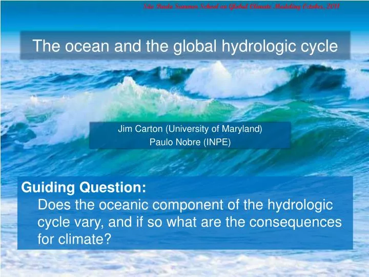
São Paulo Summer School on Global Climate Modeling October, 2011. The ocean and the global hydrologic cycle. Jim Carton (University of Maryland ) Paulo Nobre (INPE). Guiding Question: Does the oceanic component of the hydrologic cycle vary, and if so what are the consequences for climate? .

E N D
São Paulo Summer School on Global Climate Modeling October, 2011 The ocean and the global hydrologic cycle Jim Carton (University of Maryland) Paulo Nobre (INPE) Guiding Question: Does the oceanic component of the hydrologic cycle vary, and if so what are the consequences for climate?
Outline • Overview: • mean global salt and freshwater budgets • Measuring the oceanic hydrologic cycle • Observed and modeled trends • Connection between salinity trends and climate • Introduction to ocean modeling Carton
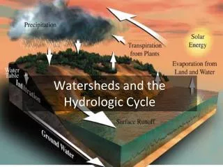
The global hydrologic cycle Carton Dai and Trenberth
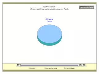
Some Numbers • Net evaporation from the ocean: 1.2 m/yr = 3.8x10⁻⁸m/s • Area of the ocean: 3.6x10¹⁴ m2 • Surface volume flux due to evap: 13.7x10⁶ m3/s or 13.7Sv (similar to the rate of formation of North Atlantic Deep Water!) • Amazon River discharge: 0.2x10⁶ m3/s (so think of evaporation as: 70 Amazons! Carton
How does this freshwater budget relate to the salinity budget? First a little math Mass is conserved, so storage and advection must balance net surface flux. The mass budget is: (1 Salinity must be conserved, but for salinity there are no sources or sinks! (except a very weak river source) (2 (2) Can be rewritten using (1) to give us the salt budget: (4 Carton Storage + advection = effective net surface flux
Climatological sea surface salinity In warm water: So, change in density due to 1psu is equivalent to 5C Carton Stephens et al., NOAA, 2002
Observed E-P Carton
Annual Range of Salinity Carton
Observing systems Carton
Present and future salinity sampling Aquarius 7dy Argo PIRATA Carton
Current Argo distribution Carton
Salinity from the PIRATA mooring at 21N, 23W: evidence of eddies! Carton
Time series at the 21N, 23W PIRATA mooring EVAP Carton
Sea surface salinity Microwave brightness temperature varies with salinity. Panel to the right shows the variations of radiation expected from a flat surface (no waves). Note that the dependence is highest at higher temperatures. Aquariusexploits this dependence to obtain an SSS measurement with an expected ~0.2PSU accuracy at monthly timescales. Lagerloef et al., 2007: The Aquarius/SAC-D Mission: Designed to Meet the Salinity Remote-Sensing Challenge, Oceanography Magazine. Carton
WOW! Carton
Trends Carton
surface salinity linear trend (psu/50yr) psu/50yr Observed 50yr drying trend over Africa Carton Durack and Wijffels (2010) Held et. al., 2005
Vertical structure of the salinity change in the Atlantic (zonally averaged) Carton
Freshening trends in the deep North Atlantic Dickson, et. al., Nature, 2002 Carton
Surface salinity change in an atmosphere-ocean coupled GCM (CM2.1) in response to elevated CO2 Carton Stouffer et al. (2006)
Salinity and climate • Heat and freshwater cycles are linked directly through the relationship between latent heat loss and evaporation: • 0.6 Sv Freshwater loss corresponds to 1.5 petawatts of latent heat flux • They are linked indirectly through the impact of salinity changes on density. Carton
Heat transport by the oceans Houghton et al., (1996: 212) Carton
Some Numbers • Assume 15Sv = 1.5x10⁶ m3/s northwards at the surface and southwards below 2000m depth • Assume a 15oC temperature difference between the two flows • The net heat transport is: • 1.5x107 x 15 x 4x106 = 0.9x10¹⁵ W! or nearly the total amount of heat being transported northwards in the North Atlantic. Carton
Freshwater transport Carton Jourdan et al., J. Phys. Oceanogr., 27, 457-467, 1997
Will the Atlantic MOC change in response to increasing greenhouse gasses? IPCC 4th Assessment Carton
Basic Equations Carton
Numerics • Arakawa-B grid in horizontal (2nd order) • Upstream advection • Leap frog time differencing • Rigid lid (w(z=0)=0) • Separate internal and extenral modes • SHMEM, MPI, shared memory, multi-threaded version Arakawa-B u,v T,S u,v u,v Carton
Our model • General circulation ocean model using POP2 numerics • Global grid • 0.1ox0.1ox42Levels (3x10⁸) • ‘Normal year’ forcing. 64yr spinup • Compute/save full salt budgets (1yr so far) • 1 year requires 12K PE hrs on an IBM Power6 10% of actual resolution Carton
Observations Model Simulation Carton
What terms balance E-P in the salt budget of the mixed layer? ? ? Do eddies contribute? Carton
Mean salt balance 0-100m average Cool color means exporting salt Carton
What we’ve learned • Oceanic hydrologic cycle overview • The oceans play a central role in the global hydrologic cycle • Patterns of surface salinity mainly reflect patterns of E-P • Observing systems: rapidly improving • ARGO born 2001 • Aquarius born 2011 • Salinity trends: • In the past 50 years salty places are getting saltier, fresh places are getting fresher • In particular, the subpolar North Atlantic has been getting fresher • These results seem to be consistent with CO2 effects based on coupled models • The implications for the meridional overturning circulation (AMOC) are still not clear • Ocean General Circulation Modeling • We’ll use this tool to look at the salt budget of the upper 100m. • High salinity ‘ocean deserts’ (source waters for the tropical thermocline) are maintained by: 1) surface evaporation, 2) poleward wind-driven transport of freshwater, and 3) horizontal eddy exchanges. How will they change? • The ‘dry’ parts of the ocean have been getting saltier possibly reflecting an intensification of the hydrologic cycle. What will this mean for Saudi Arabia? • What changes have occurred historically? • How can we improve our guesses about future conditions? • What are the impacts of these physical changes on marine biogeochemical processes? Carton
Does the oceanic component of the hydrologic cycle vary, and if so what are the consequences for climate? The answer to the first part is clearly yes. But what about the second? Carton