Download
1 / 34
380 likes | 603 Views
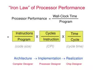
Instructions. Cycles. Time. = X X. Instruction. Program. Cycle. (code size) (CPI) (cycle time). “Iron Law” of Processor Performance. Wall-Clock Time. Processor Performance =. Program. Architecture Implementation Realization.

E N D
Instructions Cycles Time = X X Instruction Program Cycle (code size) (CPI) (cycle time) “Iron Law” of Processor Performance Wall-Clock Time Processor Performance = Program Architecture Implementation Realization Compiler Designer Processor Designer Chip Designer
Pipelined Design Motivation: Increase throughput with little increase in hardware • Bandwidth or Throughput = Performance • Bandwidth (BW) = no. of tasks/unit time • For a system that operates on one task at a time: BW = 1/ latency • BW can be increased by pipelining if many operands exist which need the same operation, i.e. many repetitions of the same task are to be performed. • Latency required for each task remains the same or may even increase slightly.
T Performance Model • Starting from an unpipelined version with propagation delay T and BW = 1/T Ppipelined=BWpipelined = 1 / (T/ k +S ) where S = delay through latch k-stage pipelined unpipelined T/k S T/k S
G Hardware Cost Model • Starting from an unpipelined version with hardware cost G Costpipelined = kL + G where L = cost of adding each latch, and k = number of stages k-stage pipelined unpipelined G/k L G/k L
Cost/Performance Trade-off [Peter M. Kogge, 1981] C/P Cost/Performance: C/P = [Lk + G] / [1/(T/k + S)] = (Lk + G) (T/k + S) = LT + GS + LSk + GT/k Optimal Cost/Performance: find min. C/P w.r.t. choice of k k
“Optimal” Pipeline Depth (kopt) x104 G=175, L=41, T=400, S=22 Cost/Performance Ratio (C/P) G=175, L=21, T=400, S=11 Pipeline Depth k
Pipelining Idealism • Uniform Suboperations The operation to be pipelined can be evenly partitioned into uniform-latency suboperations • Repetition of Identical Operations The same operations are to be performed repeatedly on a large number of different inputs • Repetition of Independent Operations All the repetitions of the same operation are mutually independent, i.e. no data dependence and no resource conflicts Good Examples: automobile assembly line floating-point multiplier instruction pipeline???
Instruction Pipeline Design • Uniform Suboperations ... NOT! balance pipeline stages - stage quantization to yield balanced stages - minimize internal fragmentation (some waiting stages) • Identical operations ... NOT! unifying instruction types - coalescing instruction types into one “multi-function” pipe - minimize external fragmentation (some idling stages) • Independent operations ... NOT! resolve data and resource hazards - inter-instruction dependency detection and resolution - minimize performance lose
The Generic Instruction Cycle • The “computation” to be pipelined • Instruction Fetch (IF) • Instruction Decode (ID) • Operand(s) Fetch (OF) • Instruction Execution (EX) • Operand Store (OS) • Update Program Counter (PC)
Based on Obvious Subcomputations: The GENERIC Instruction Pipeline (GNR)
IF ID OF EX OS Balancing Pipeline Stages • Without pipelining Tcyc TIF+TID+TOF+TEX+TOS = 31 • Pipelined Tcyc max{TIF, TID, TOF, TEX, TOS} = 9 Speedup= 31 / 9 Can we do better in terms of either performance or efficiency? TIF= 6 units TID= 2 units TID= 9 units TEX= 5 units TOS= 9 units
Balancing Pipeline Stages • Two Methods for Stage Quantization: • Merging of multiple subcomputations into one. • Subdividing a subcomputation into multiple subcomputations. • Current Trends: • Deeper pipelines (more and more stages). • Multiplicity of different (subpipelines). • Pipelining of memory access (tricky).
Granularity of Pipeline Stages Coarser-Grained Machine Cycle: 4 machine cyc / instruction cyc Finer-Grained Machine Cycle: 11 machine cyc /instruction cyc TIF&ID= 8 units TID= 9 units TEX= 5 units TOS= 9 units Tcyc= 3 units
Hardware Requirements • Logic needed for each pipeline stage • Register file ports needed to support all the stages • Memory accessing ports needed to support all the stages
IF IF PC GEN IF 1 PC GEN . Cache Read ID PC GEN . Cache Read PC GEN . RD 2 OF Decode ID PC GEN . Read REG OF PC GEN . EX ALU 3 Add GEN PC GEN . Cache Read PC GEN . Cache Read MEM 4 OS PC GEN . EX 1 EX PC GEN . EX 2 PC GEN . WB 5 OS Write Result PC GEN . Pipeline Examples MIPS R2000/R3000 AMDAHL 470V/7 1 2 3 4 5 6 7 8 9 10 Check Result 11 PC GEN . 12
Unifying Instruction Types • Procedure: • Analyze the sequence of register transfers required by each instruction type. • Find commonality across instruction types and merge them to share the same pipeline stage. • If there exists flexibility, shift or reorder some register transfers to facilitate further merging.
The 6-stage TYPICAL (TYP) pipeline: Coalescing Resource Requirements
IF ALU Instruction Flow Path
IF Load Instruction Flow Path
IF Store Instruction Flow Path What is wrong in this figure?
IF Branch Instruction Flow Path
Pipelining: Steady State t0 t1 t2 t3 t4 t5 Insti IF ID RD ALU MEM WB Insti+1 IF ID RD ALU MEM WB Insti+2 IF ID RD ALU MEM WB Insti+3 IF ID RD ALU MEM Insti+4 IF ID RD ALU IF ID RD IF ID F
Instruction Dependencies • Data Dependence • True dependence (RAW) Instruction must wait for all required input operands • Anti-Dependence (WAR) Later write must not clobber a still-pending earlier read • Output dependence (WAW) Earlier write must not clobber an already-finished later write • Control Dependence (aka Procedural Dependence) • Conditional branches cause uncertainty to instruction sequencing • Instructions following a conditional branch depends on the resolution of the branch instruction (more exact definition later)
bge $10, $9, $36 mul $15, $10, 4 addu $24, $6, $15 lw $25, 0($24) mul $13, $8, 4 addu $14, $6, $13 lw $15, 0($14) bge $25, $15, $36 $35: addu $10, $10, 1 . . . $36: addu $11, $11, -1 . . . Example: Quick Sort on MIPS R2000 • # for (;(j<high)&&(array[j]<array[low]);++j); • # $10 = j; $9 = high; $6 = array; $8 = low
Sequential Code Semantics Instruction Dependences and Pipeline Hazards A true dependence between two instructions may only involve one subcomputation of each instruction. i1: xxxx i1 i1: i2: xxxx i2 i2: i3: xxxx i3 i3: The implied sequential precedences are overspecifications. It is sufficient but not necessary to ensure program correctness.
Necessary Conditions for Data Hazards stage X j:rk_ Reg Write j:rk_ Reg Write j:_rk Reg Read iOj iAj iDj stage Y Reg Write Reg Read Reg Write i:rk_ i:_rk i:rk_ WAW Hazard WAR Hazard RAW Hazard dist(i,j) dist(X,Y) ?? dist(i,j) > dist(X,Y) ?? dist(i,j) dist(X,Y) Hazard!! dist(i,j) > dist(X,Y) Safe


![[Post Processor]](https://cdn2.slideserve.com/5127715/slide1-dt.jpg)