Download
1 / 30
300 likes | 418 Views
Emergence of Coherence and Scaling in an Ensemble of Globally Coupled Chaotic Systems. Sang-Yoon Kim Department of Physics Kangwon National University. Globally Coupled Systems (Each element is coupled to all the other ones with equal strength). Synchronized Flashing of Fireflies.

E N D
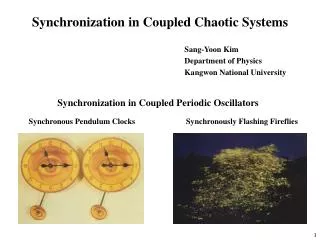
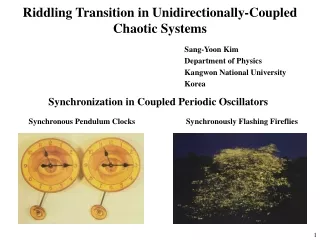
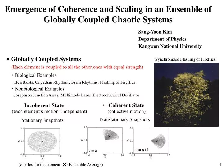
Emergence of Coherence and Scaling in an Ensemble of Globally Coupled Chaotic Systems Sang-Yoon Kim Department of Physics Kangwon National University • Globally Coupled Systems (Each element is coupled to all the other ones with equal strength) Synchronized Flashing of Fireflies Biological Examples Heartbeats, Circadian Rhythms, Brain Rhythms, Flashing of Fireflies Nonbiological Examples Josephson Junction Array, Multimode Laser, Electrochemical Oscillator Coherent State Incoherent State (each element’s motion: independent) (collective motion) Nonstationary Snapshots Stationary Snapshots t = n+1 t = n (i: index for the element, : Ensemble Average)
Emergent Science “The Whole is Greater than the Sum of the Parts.” Complex Nonlinear Systems: Spontaneous Emergence of Dynamical Order Order Parameter ~ 1 Order Parameter ~ 0 Order Parameter < 1 2
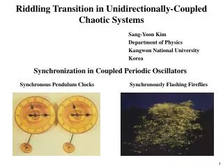
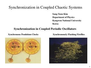
Two Mechanisms for Synchronous Rhythms Leading by a Pacemaker • Collective Behavior of All Participants
Synchronization of Pendulum Clocks Synchronization by Weak Coupling Transmitted through the Air or by Vibrations in the Wall to which They are Attached First Observation of Synchronization by Huygens in Feb., 1665
Circadian Rhythms Growth Hormone (ng/mL) Temperature (ºc) Time of day (h) Time of day (h) • Biological Clock Ensemble of Neurons in the Suprachiasmatic Nuclei (SCN) Located within the Hypothalamus: Synchronization → Circadian Pacemaker [Zeitgebers (“time givers”): light/dark] 5
Integrate and Fire (Relaxation) Oscillator Mechanical Model for the IF Oscillator water level time water outflow Accumulation (Integration) “Firing” time Van der Pol (Relaxation) Oscillator Firings of a Pacemaker Cell in the Heart Neuron Firings of a Neuron
Synchronization in Pulse-Coupled IF Oscillators Population of Globally Pulse-Coupled IF Oscillators [Lapicque, J. Physiol. Pathol. Gen. 9, 620 (1971)] Kicking Full Synchronization Heart Beat:Stimulated by the Sinoatrial (SN) Node Located on the Right Atrium, Consisting of Pacemaker Cells [R. Mirollo and S. Strogatz, SIAM J. Appl. Math. 50, 1645 (1990)]
Emergence of Dynamical Order and Scaling in A Large Population of Globally Coupled Chaotic Systems • Scaling Associated with Coherence with a Macroscopic • Mean Field Successive Appearance of Similar • Coherent States of Higher Order
Period-Doubling Route to Chaos Lorenz Attractor [Lorenz, J. Atmos. Sci. 20, 130 (1963)] Butterfly Effect [Small Cause Large Effect] Sensitive Dependence on Initial Conditions Logistic Map [May, Nature 261, 459 (1976)] : Representative Model for Period-Doubling Systems Transition to Chaos at a Critical Point a* (=1.401 155 189 …) via an Infinite Sequence of Period Doublings : Lyapunov Exponent (exponential divergence rate of nearby orbits) 0 Regular Attractor > 0 Chaotic Attractor 9
Universal Scaling Associated with Period Doublings Noisy Logistic Map Universal Scaling Factors: =4.669 201 … =-2.502 987 … =6.619 03 [ M.J. Feigenbaum, J. Stat. Phys. 19, 25 (1978), J. Crutchfield, M. Nauenberg, and J. Rudnick, Phys. Rev. Lett. 46, 459 (1981). B. Shraiman, C.E. Wayne, and P.C. Martine, Phys. Rev. Lett. 46, 462 (1981).] Parametrically Forced Pendulum [S.-Y. Kim and K. Lee, Phys. Rev. E 53, 1579 (1996).] w: Gaussian White Noise with <w(t)>=0 and <w(t1) w(t2)> = (t1 – t2). h(t)=Acos(2t) -A* (=2, =1, A* = 6.57615 …)
Globally Coupled Noisy Chaotic Systems An Ensemble of Globally Coupled Noisy Logistic Maps Uniform Random Noise with a Zero Mean and Unit Variance Parameter to Control the Noise Strength • A Population of 1D Chaotic Maps Interacting via the Mean Field: • Dissipative Coupling Tending to Equalize the States of Elements Main Interest Investigation: Coherence in Asynchronous Chaotic Attractors and Scaling Associated with the Mean Field
Scaling near the Zero-Coupling Critical Point (N=10 ) 4 Universal Scaling near the Zero-Coupling Critical Point (a, , ) = (a*, 0, 0): (a* = 1.401 155 189 …) • Dynamical Behavior at a Set of Parameters (a, , ) • Dynamical Behavior [with Doubled Time Scale (t=2)] at a Set of Renormalized Parameters (a/, /c, /) [=4.669201, =6.61903] “Scaling Factor for the Coupling Parameter for the Dissipative Coupling: Asynchronous Chaotic Attractors (containing the diagonal) [ Renormalization Results: 1. S.P.Kuznetsov, Radiophysics and Quantum Electronics 28, 681 (1985). 2. S.-Y. Kim and H. Kook, Phys. Rev. E 48, 785 (1993). 3. S.-Y. Kim and H. Kook, Phys. Lett. A 178, 258 (1993).]
Coherent and Incoherent States Ensemble-Averaged Mean Field h(t) In the Thermodynamic Limit of N→∞, Incoherent State (Each Element: Independent Motion) Coherent State (Collective Motion) Multiple Transitions to Coherence for Incoherent State (Gray, ε=0.02) Coherent State (Black, ε=0.03)
Mean- Field Dynamic of Asynchronous Chaotic Attractors for Δa=0.32 ε=0.03 ε=0.02 ε=0.03 ε=0.033 ε=0.035 ε=0.036 ε=0.033 ε=0.035 ε=0.036
Order Parameter for the Coherent Transition Order Parameter Variance (Mean Square Deviation) of the Mean Field h(t) In the Thermodynamic Limit of N→∞, > 0 for the Coherent State → 0 for the Incoherent State ∆a=0.32, σ=0.001 ∆ ε Incoherent State Coherent State ε ε*~0.0291
x=1 (most concentrated region) x=0 (most rarified region) Scaling for the Mean Field : Exhibiting the ‘2’-scaling (=-2.502 987 …) Mean Field Return Maps of the Mean Field for Orbital Scalings in the Logistic Map h(2 τ+1)) τ a=0.32/i, =0.02/2i, =0.001/i, t =2i [i (level of renormalization)=0, 1, 2] • ‘’-scaling near the Critical Point x=0 • ‘2’-scaling near the First Iterate of the Critical Point x=1 [= f(0)]
4 Appearance of Similar Coherent States of Higher Orders (N=10 ) 1st-Order Renormalized State (a=0.32/, =0.001/) Return Map Bifurcation Diagram Variance Diagram =0.039/2 2nd-Order Renormalized State (a=0.32/2, =0.001/2) =0.039/22 3rd-Order Renormalized State (a=0.32/3, =0.001/3) =0.039/23
Self-Similar State Diagrams (N=10 ) 4 =0.001 Incoherent States (White) Coherent States (Gray) 1st Renormalized State Diagram 2nd Renormalized State Diagram =0.001/ =0.001/2
Effect of Noise on the Transition to Coherence 0th Order State Diagram • Multiple Transitions to Coherence for < * (=0.003) • Single Period-Doubling Transition to Coherence for > * Scaling for the State Diagram in the - Plane 1st Order Renormalized State Diagram 2nd Order Renormalized State Diagram a=0.32/ a=0.32/2
A Global Population of Inertially Coupled Maps Renormalization Result for the Scaling of the Coupling Parameter: [Renormalization Results: S.P.Kuznetsov, Radiophysics and Quantum Electronics 28, 681 (1985). S.-Y. Kim and H. Kook, Phys. Rev. E 48, 785 (1993). S.-Y. Kim and H. Kook, Phys. Lett. A 178, 258 (1993).] • Nonlinear Coupling [Tendency of equalizing the states of the elements Dissipative coupling] One Relevant Scaling Factor: =2 • Linear Coupling Two Relevant Scaling Factors: 1 = (=-2.502 987 …): inertial coupling (each element: maintaining the memory of its previous states) 2 = 2 • Combination of the Linear and Quadratic Coupling [Ref: S.P. Kuznetsov, Chaos, Solitons, and Fractals 2, 281-301 (1992).] Pure Inertial Coupling with Only One Relevant Scaling Factor: =
Scaling near the Zero-Coupling Critical Point (N=10 ) 4 Universal Scaling near the Zero-Coupling Critical Point (a, , ) = (a*, 0, 0): (a* = 1.401 155 189 …) • Dynamical Behavior at a Set of Parameters (a, , ) • Dynamical Behavior [with Doubled Time Scale (t=2)] at a Set of Renormalized Parameters (a/, /c, /) [=4.669201, =6.61903] “Scaling Factor for the Coupling Parameter for the Inertial Coupling: Asynchronous Chaotic Attractors (containing the diagonal) [ Renormalization Results: 1. S.P.Kuznetsov, Radiophysics and Quantum Electronics 28, 681 (1985). 2. S.-Y. Kim and H. Kook, Phys. Rev. E 48, 785 (1993). 3. S.-Y. Kim and H. Kook, Phys. Lett. A 178, 258 (1993).]
Onset of Coherence Bifurcation Diagram and Return Map of the Mean Field k(t) (N=10 ) 4 Coherent State for ε=0.04 Incoherent State for ε=0.02 Δa=0.32 σ=0.003 Order Parameter Coherent Incoherent Coherent
x=1 (most concentrated region) x=0 (most rarified region) Scaling for the Mean Field Mean Field : Exhibiting the ‘’-scaling (=-2.502 987 …) Return Maps of the Mean Field for Orbital Scalings in the Logistic Map a=0.32/i, =0.02/2i, =0.003/i, t =2i [i (level of renormalization)=0, 1, 2] • ‘’-scaling near the Critical Point x=0
Scaling Associated with the Mean Field k(t) (N=10 ) 4 1st-Order Renormalized State (a=0.32, =0.003) Bifurcation Diagram Variance Diagram Return Map =0.04 2nd-Order Renormalized State (a=0.32/, =0.003/) =0.04/ 3rd-Order Renormalized State (a=0.32/2, =0.003/2) =0.04/2
Coherence and Scaling in a Heterogeneous Ensemble of Globally Coupled Maps Heterogeneous Ensemble (consisting of non-identical elements) Spread in the map parameter ai for each element: Randomly chosen with uniform distribution in the interval of (a-, a+) (: spread parameter) Transition from an Incoherent to a Coherent State Occurrence of a Coherence at =* (=0.0289) for a=0.32 and =0.006 Coherent State for =0.03 Incoherent State for ε=0.02
Successive Appearance of Similar Coherent States of Higher Orders 1st-Order Renormalized State (a=0.32/, =0.006/) Variance Diagram Return Map Bifurcation Diagram =0.038/2 2nd-Order Renormalized State (a=0.32/2, =0.006/2) =0.038/22 3rd-Order Renormalized State (a=0.32/3, =0.006/3) =0.038/23
An Ensemble of Globally Coupled Noisy Pendulums Globally Coupled Noisy Pendulums Phase Coherent Attractor in the Single Pendulum =2, =1 A(A-A*)=0.06 (A*=6.57615) =0.0015 • Phase Coherence (Flow) and Amplitude Incoherence A=0.06 =0.0015 =0.2 • Mean Field: Rotation on a Noisy Limit Cycle (Flow), Noisy Stationary State (Map)
Onset of Coherence Bifurcation Diagram and Return Map of the Mean Field H(n)(N=10 ) 4 Coherent State for ε=0.04 Incoherent State for ε=0.02 Order Parameter Incoherent Coherent
=0.3/2 2 =0.3/2 3 Scaling Associated with the Mean Field H(n) (N=10 ) 4 1st-Order Renormalized State (A=0.06/, =0.0015/) Bifurcation Diagram MSD Diagram Return Map =0.3/2 2nd-Order Renormalized State (A=0.06/2, =0.0015/2) 3rd-Order Renormalized State (A=0.06/3, =0.0015/3)
Summary • Investigation of Onset of Coherence in an Ensemble of Globally Coupled Noisy Logistic Maps (a, , ) (a*, 0, 0): zero-coupling critical point Successive Appearance of Similar Coherent States of Higher Orders Universality for the Results Confirmed in a Population of Globally Coupled Noisy Pendulums • Our Results: Valid in an Ensemble of Globally Coupled Period-Doubling Systems of Different Nature