Download
1 / 17
170 likes | 183 Views
Introduction to Graph Theory. Lecture 11: Eulerian and Hamiltonian Graphs. Hamiltonicity. As opposed to Eulerian graphs, we now want to make sure we visit each vertex just once. The famous application for such a graph is the traveling salesman problem

E N D
Introduction to Graph Theory Lecture 11: Eulerian and Hamiltonian Graphs
Hamiltonicity • As opposed to Eulerian graphs, we now want to make sure we visit each vertex just once. • The famous application for such a graph is the traveling salesman problem • Starting from the home city, the salesman should visit each city to show his merchandise.
Terminology • A graph with a spanning path is called traceable. • A graph with a spanning cycle is called hamiltonian. • The spanning cycle is called hamiltonian cycle. • A traceable non-hamiltonian graph is called semi-hamiltonian • Having only hamiltonian path, not cycle
Observations • Unlike eulerian graphs, it is often hard to determine if a graph is hamiltonian. • Some necessary conditions for a graph to be hamiltonian • If graph G is bipartite, but not equitable, then not hamiltonian. • The graph must be 2-connected (no cut vertex) • Can we see why?
Hamiltonicity of Hypercubes • Hamiltonicity of a constructed graph can be derived from the component graphs. • : consisting of 2 copies of G (G and G’). If G is traceable, then is hamiltonian. • Taking the spanning path P in G with endpoint x and y • Taking its mirror image path P’ in G’ with endpoint x’ and y’ • Adding xx’ and yy’ to the path • is hamiltonian, so are
Sufficient Conditions • There exist many such conditions that guarantee that a given graph is hamiltonian. • We just study one of them (popular and easier) • Theorem 5.2: If G is a graph of order such that , then G is hamiltonian.
Proof of Theorem 5.2 • If n=3, then implies that , which is hamiltonian. • Now suppose n>3 and let be a path of maximum length in G • Observation1: Since , P must contain at least vertices. Reason: The only possible additional adjacencies of v1 and vklie within the set • Observation2: There must be some vertex such that and are adjacent while and are adjacent.
(cont) • Now we know that G contains a cycle • Suppose If there is a vertex u not in C. Using observation1, u must be adjacent to at least one vertex on C => a longer path than P. Therefore impossible. • Therefore C contains all vertices, and thusa hamiltonian cycle.
Some Remarks • The converse of Theorem is not true. • If G is hamiltonian, it needs not have the property • Take for as an example • Can you tell the difference between necessary and sufficient conditions?
Homogeneous Connected • Given any vertex , there exists a hamiltonian path starting at v. • Hamiltonian graph is homogeneous connected. • Simply by deleting an edge of the spanning cycle incident with v. • Please note that the reverse is not always true. • E.g Peterson graph
Hamiltonian Connected • Given any pair of vertices x and y, there is an x-y halmiltonian path for G • For example, • If G is hamiltonian connected, it is homogenous connected • If order is at least 3, a hamiltonian-connected => hamiltonian • Proof?
Hypercubes • We know that are hamiltonian for • But hypercubes are not hamiltonian connected • Picking any two vertices x and y of the same color. in the bipartite hypercube. • has even order, thus the hamiltonian path is even order with end vertices of opposite colors • Therefore, there is no x-y hamiltonian path. • But are hamilton laceable.
Hamilton Laceble • An equitable bipartite graph G is hamilton laceble if there exists an x-y spanning path for G for any two oppositely colored vertices x and y. • Theorem 5.4: is hamilton laceable • Proof by induction (some typos in the textbook)
Proof of Theorem 5.4 • Basic case: true for n=1 or 2. • Hypothesis: Assume true for n=k (Qk) • Prove that the theorem is true for n=k+1 (Qk+1) • Let r and b be vertices of Qk+1, s.t. r is red and b is blue. • Split Qk+1 into two copies of Qk, R and B, such that • We know that R is hamiltonian and bipartite, so there exists a cycle spanning C containing r and its neighbor x. • Let x’ be a neighbor of x in B. Since x is blue, x’ must be red. • By the hypothesis, we can find an b-x’ spanning path L in B. • The required r-b spanning path for Qk+1 is M, xx’,L, where M is the spanning path from r to x on C.
Application: The Traveling Salesman • We want to find the hamiltonian cycle of minimum weight --- least cost b 5 c 3 a 3 6 4 2 8 d 2 7 f 3 e
Some Remarks • In applications the problems are much more overwhelming • There is no efficient method for solving the traveling salesman problem • There are approximation techniques for this problem • The problem is intrinsically difficult to solve.
Term Project • Available online now.